By Flavio De Stefano
It was 4 years ago when I had the idea to replicate the Apple® Siri wave-form (introduced with the iPhone 4S) in the browser using pure Javascript.
During the last month, I updated this library by doing a lot of refactoring using ES6 features and reviewed the build process using RollupJS. Now I’ve decided to share what I've learned during this process and the math behind this library.
To get an idea what the output will be, visit the live example; the whole codebase is here.
Additionally, you can download all plots drawn in this article in GCX (OSX Grapher format): default.gcx and ios9.gcx.
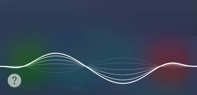
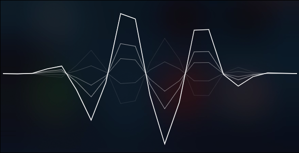
The classic wave style
Initially, this library only had the classic wave-form style that all of you remember using in iOS 7 and iOS 8.
It’s no hard task to replicate this simple wave-form, only a bit of math and basic concepts of the Canvas API.
You’re probably thinking that the wave-form is a modification of the Sine math equation, and you're right…well, almost right.
Before starting to code, we’ve got to find our linear equation that will be simply applied afterwards. My favourite plot editor is Grapher; you can find it in any OSX installation under _Applications > Utilities > Graphe_r.app.
We start by drawing the well known:
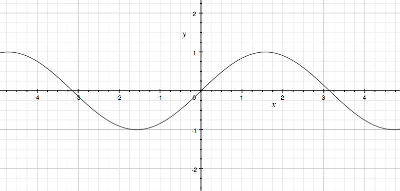
Perfecto! Now, let’s add some parameters (Amplitude [A], Time coordinate[t] and Spatial frequency [k]) that will be useful later (Read more here: https://en.wikipedia.org/wiki/Wave).
Now we have to “attenuate” this function on plot boundaries, so that for |x| >; 2, the y values tends to 0. Let’s draw separately an equation g(x) that has these characteristics.
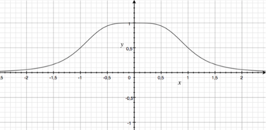
This seems to be a good equation to start with. Let’s add some parameters here too to smooth the curve for our purposes:
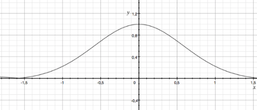
Now, by multiplying our f(x, …) and g(x, …), and by setting precise parameters to the other static values, we obtain something like this.
- A = 0.9 set the amplitude of the wave to max Y = A
- k = 8 set the spatial frequency and we obtain “more peaks” in the range [-2, 2]
- t = -π/2 set the phase translation so that f(0, …) = 1
- K = 4 set the factor for the “attenuation equation” so that the final equation is y = 0 when |x| ≥ 2
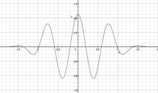
It looks good! ?
Now, if you notice on the original wave we have other sub-waves that will give a lower value for the amplitude. Let’s draw them for A = {0.8, 0.6, 0.4, 0.2, -0.2, -0.4, -0.6, -0.8}
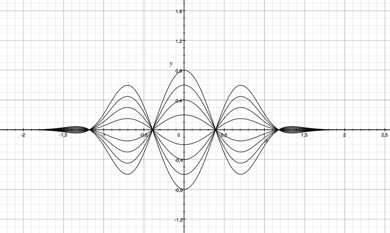
In the final canvas composition the sub-waves will be drawn with a decreasing opacity tending to 0.
Basic code concepts
What do we do now with this equation?
We use the equation to obtain the Y value for an input X.
Basically, by using a simple for loop from -2 to 2, (the plot boundaries in this case), we have to draw point by point the equation on the canvas using the beginPath and lineTo API.
const ctx = canvas.getContext('2d');
ctx.beginPath();ctx.strokeStyle = 'white';
for (let i = -2; i <= 2; i += 0.01) { const x = _xpos(i); const y = _ypos(i); ctx.lineTo(x, y);}
ctx.stroke();
Probably this pseudo-code will clear up these ideas. We still have to implement our _xpos and _ypos functions.
But… hey, what is 0.01⁉️ That value represents how many pixels you move forward in each iteration before reaching the right plot boundary… but what is the correct value?
If you use a really small value (<0.01), you’ll get an insanely precise rendering of the graph but your performance will decrease because you’ll get too many iterations.
Instead, if you use a really big value (> 0.1) your graph will lose precision and you’ll notice this instantly.
You can see that the final code is actually similar to the pseudo-code: https://github.com/kopiro/siriwave/blob/master/src/curve.js#L25
Implement _xpos(i)
You may argue that if we’re drawing the plot by incrementing the x, then _xpos may simply return the input argument.
This is almost correct, but our plot is always drawn from -B to B (B = Boundary = 2).
So, to draw on the canvas via pixel coordinates, we must translate -B to 0, and B to 1 (simple transposition of [-B, B] to [0,1]); then multiply [0,1] and the canvas width (w).
_xpos(i) = w * [ (i + B) / 2B ]
https://github.com/kopiro/siriwave/blob/master/src/curve.js#L19
Implement _ypos
To implement _ypos, we should simply write our equation obtained before (closely).
const K = 4;const FREQ = 6;
function _attFn(x) { return Math.pow(K / (K + Math.pow(x, K)), K);}
function _ypos(i) { return Math.sin(FREQ * i - phase) * _attFn(i) * canvasHeight * globalAmplitude * (1 / attenuation);}
Let’s clarify some parameters.
- canvasHeight is Canvas height expressed in PX
- i is our input value (the x)
- phase is the most important parameter, let’s discuss it later
- globalAmplitude is a static parameter that represents the amplitude of the total wave (composed by sub-waves)
- attenuation is a static parameter that changes for each line and represents the amplitude of a wave
https://github.com/kopiro/siriwave/blob/master/src/curve.js#L24
Phase
Now let’s discuss about the phase variable: it is the first changing variable over time, because it simulates the wave movement.
What does it mean? It means that for each animation frame, our base controller should increment this value. But to avoid this value throwing a buffer overflow, let’s modulo it with 2π (since Math.sin dominio is already modulo 2π).
phase = (phase + (Math.PI / 2) * speed) % (2 * Math.PI);
We multiply speed and Math.PI so that with speed = 1 we have the maximum speed (why? because sin(0) = 0, sin(π/2) = 1, sin(π) = 0, … ?)
Finalizing
Now that we have all code to draw a single line, we define a configuration array to draw all sub-waves, and then cycle over them.
return [ { attenuation: -2, lineWidth: 1.0, opacity: 0.1 }, { attenuation: -6, lineWidth: 1.0, opacity: 0.2 }, { attenuation: 4, lineWidth: 1.0, opacity: 0.4 }, { attenuation: 2, lineWidth: 1.0, opacity: 0.6},
// basic line { attenuation: 1, lineWidth: 1.5, opacity: 1.0},];
https://github.com/kopiro/siriwave/blob/master/src/siriwave.js#L190
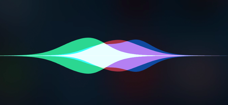
The iOS 9+ style
Now things start to get complicated. The style introduced with iOS 9 is really complex and the reverse engineering to simulate it it’s not easy at all! I’m not fully satisfied of the final result, but I’ll continue to improve it until I get the desired result.
As previously done, let’s start to obtain the linear equations of the waves.

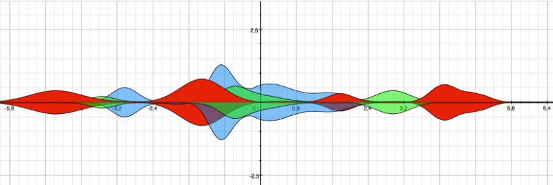
As you can notice:
- we have three different specular equations with different colours (green, blue, red)
- a single wave seems to be a sum of sine equations with different parameters
- all other colours are a composition of these three base colours
- there is a straight line at the plot boundaries
By picking again our previous equations, let’s define a more complex equation that involves translation. We start by defining again our attenuation equation:
Now, define h(x, A, k, t) function, that is the sine function multiplied for attenuation function, in its absolute value:
We now have a powerful tool.
With h(x), we can now create the final wave-form by summing different h(x) with different parameters involving different amplitudes, frequency and translations. For example, let’s define the red curve by putting random values.
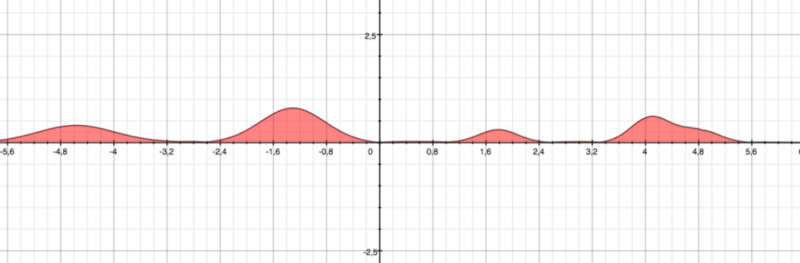
If we do the same with a green and blue curve, this is the result:
This is not quite perfect, but it could work.
To obtain the specular version, just multiply everything by -1.
In the coding side, the approach is the same, we have only a more complex equation for _ypos.
const K = 4;const NO_OF_CURVES = 3;
// This parameters should be generated randomlyconst widths = [ 0.4, 0.6, 0.3 ];const offsets = [ 1, 4, -3 ];const amplitudes = [ 0.5, 0.7, 0.2 ];const phases = [ 0, 0, 0 ];
function _globalAttFn(x) { return Math.pow(K / (K + Math.pow(x, 2)), K);}
function _ypos(i) { let y = 0; for (let ci = 0; ci < NO_OF_CURVES; ci++) { const t = offsets[ci]; const k = 1 / widths[ci]; const x = (i * k) - t; y += Math.abs( amplitudes[ci] * Math.sin(x - phases[ci]) * _globalAttFn(x) ); }
y = y / NO_OF_CURVES; return canvasHeightMax * globalAmplitude * y;}
There’s nothing complex here. The only thing that changed is that we cycle NO_OF_CURVES times over all pseudo-random parameters and we sum all y values.
Before multiplying it for canvasHeightMax and globalAmplitude that give us the absolute PX coordinate of the canvas, we divide it for NO_OF_CURVES so that y is always ≤ 1.
https://github.com/kopiro/siriwave/blob/master/src/ios9curve.js#L103
Composite operation
One thing that actually matters here is the globalCompositeOperation mode to set in the Canvas. If you notice, in the original controller, when there’s a overlap of 2+ colors, they’re actually mixed in a standard way.
The default is set to source-over, but the result is poor, even with an opacity set.

You can see all examples of vary globalCompositeOperation here: https://developer.mozilla.org/en-US/docs/Web/API/CanvasRenderingContext2D/globalCompositeOperation
By setting globalCompositeOperation to “ligther”, you notice that the intersection of the colours is nearest to the original.

Build with RollupJS
Before refactoring everything, I wasn’t satisfied at all with the codebase: old prototype-like classes, a single Javascript file for everything, no uglify/minify and no build at all.
Using the new ES6 feature like native classes, spread operators and lambda functions, I was able to clean everything, split files, and decrease lines of unnecessary code.
Furthermore, I used RollupJS to create a transpiled and minified build in various formats.
Since this is a browser-only library, I decided to create two builds: an UMD (Universal Module Definition) build that you can use directly by importing the script or by using CDN, and another one as an ESM module.
The UMD module is built with this configuration:
{ input: 'src/siriwave.js', output: { file: pkg.unpkg, name: pkg.amdName, format: 'umd' }, plugins: [ resolve(), commonjs(), babel({ exclude: 'node_modules/**' }), ]}
An additional minified UMD module is built with this configuration:
{ input: 'src/siriwave.js', output: { file: pkg.unpkg.replace('.js', '.min.js'), name: pkg.amdName, format: 'umd' }, plugins: [ resolve(), commonjs(), babel({ exclude: 'node_modules/**' }), uglify()]}
Benefiting of UnPKG service, you can find the final build on this URL served by a CDN: https://unpkg.com/siriwave/dist/siriwave.min.js
This is the “old style Javascript way” — you can just import your script and then refer in your code by using SiriWave global object.
To provide a more elegant and modern way, I also built an ESM module with this configuration:
{ input: ‘src/siriwave.js’, output: { file: pkg.module, format: ‘esm’ }, plugins: [ babel({ exclude: ‘node_modules/**’ }) ]}
We clearly don’t want the resolve or commonjs RollupJS plugins because the developer transplier will resolve dependencies for us.
You can find the final RollupJS configuration here: https://github.com/kopiro/siriwave/blob/master/rollup.config.js
Watch and Hot code reload
Using RollupJS, you can also take advantage of rollup-plugin-livereload and rollup-plugin-serve plugins to provide a better way to work on scripts.
Basically, you just add these plugins when you’re in “developer” mode:
import livereload from 'rollup-plugin-livereload';import serve from 'rollup-plugin-serve';
if (process.env.NODE_ENV !== 'production') { additional_plugins.push( serve({ open: true, contentBase: '.' }) ); additional_plugins.push( livereload({ watch: 'dist' }) );}
We finish by adding these lines into the package.json:
"module": "dist/siriwave.m.js","jsnext:main": "dist/siriwave.m.js","unpkg": "dist/siriwave.js","amdName": "SiriWave","scripts": { "build": "NODE_ENV=production rollup -c", "dev": "rollup -c -w"},
Let’s clarify some parameters:
- module / jsnext:main: path of dist ESM module
- unpkg: path of dist UMD module
- amdName: name of the global object in UMD module
Thanks a lot RollupJS!
Hope that you find this article interesting, see you soon! ?