
A straight line equation is a good place to start understanding how a neural network works. It's what we explored in my previous article, How Neural Networks Work – Explained Using the Straight Line Equation (y=ax+b).
But, what if the relationship between the input and the output isn't linear?
We all know that in the real world, the data doesn't always follow a straight line pattern. This is where things start getting interesting: sometimes a single rule isn't enough to describe the relationship between the variables.
That’s where non-linearity comes in. It allows neural networks to capture changing behaviour in data.
In this article, we'll explore the concept of non-linearity that can capture complex relationships in data. Using a simple example, we'll try to understand piecewise linear curves, ReLU functions, S-shaped curves, and sigmoid functions in relation to how they help neural networks learn patterns that a straight line can't describe.
Table of Contents
Prerequisites
Basic understanding of linear functions
Familiarity with the concept of deep neural networks
When a Straight Line Is Enough
A straight line equation means that the same rule applies throughout the relationship.
y = ax + b
y => Output variable
x => Input variable
a => Amount by which y changes when x changes (slope)
b => Value of y when x is 0 (y intercept)
We can look at an example to understand it better.
Ms. Poly is a math teacher who wants to come up with a study plan for her students to help them ace the final exam. She creates a rule of thumb using one factor: the number of hours studied per week. This means that the mark scored by a student is directly proportionate to the hours they spend studying.
Based on her assumption, she comes up with an equation in the form y=ax+b.
y => Marks scored
x => Number of hours studied
a => Increase in marks for every hour studied
b => Minimum marks every student is capable of scoring without studying.
So, after a quarterly exam, she interviews her students and collects information on how many hours they studied math per week. She creates a table with two columns: number of hours studied (x) per week and marks scored (y) and plots them.
| Number of Hours Studied | Marks Scored |
|---|---|
| 0 | 40 |
| 1 | 40 |
| 2 | 41 |
| 3 | 40 |
| 4 | 48 |
| 5 | 58 |
| 6 | 69 |
| 7 | 80 |
| 8 | 80 |
But when she tries to apply her simple formula, it doesn't seem to align with the data she collected, proving that real-life data is rarely that straightforward.
When a Straight Line Isn't Enough
Ms. Poly observes the graph closely and identifies a few patterns. Students who study for only a few hours may not see much improvement. Once they cross a certain point, their marks begin to increase with additional study. And again after a certain point, the marks remain fairly constant.
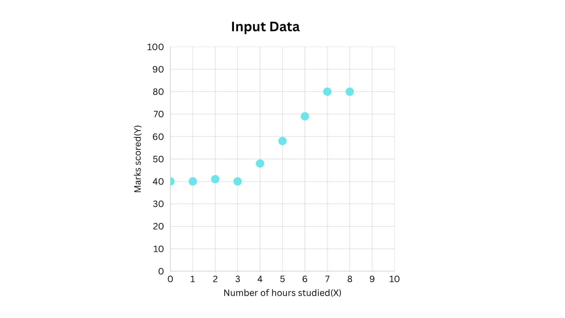
Thus, Ms Poly’s simple straight line equation isn’t enough to describe the relation between number of hours studied (x) per week and marks scored (y).
Instead, it can be divided into three parts,
Less than t₁ hours: Marks remain constant
t₁ to t₂ hours: Marks increase with study time
More than t₂ hours: Marks remain constant
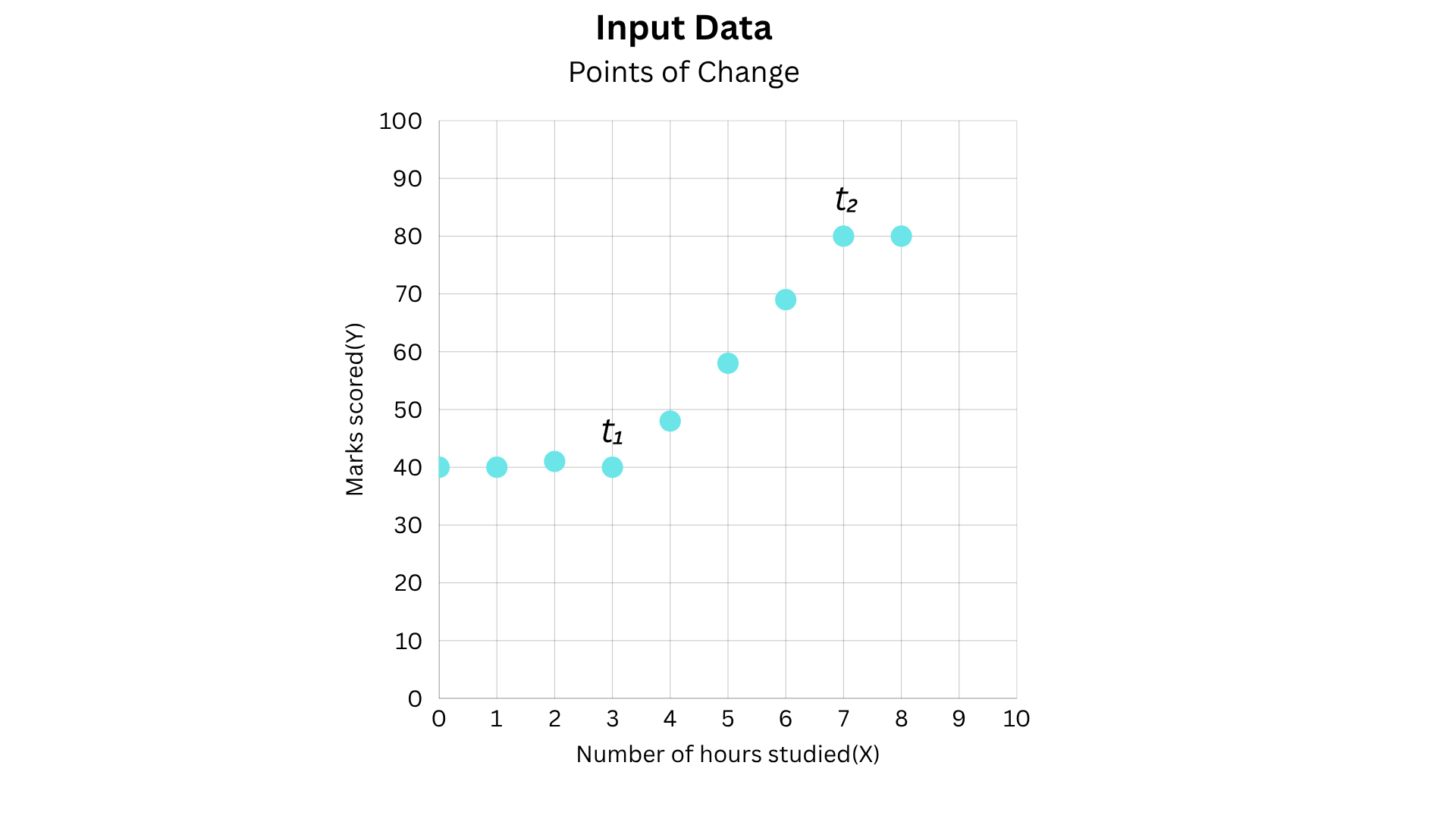
So, she can have separate equations for each range and write them like this:
y = 1st equation, x<t₁
y = 2nd equation, t₁<=x<t₂
y = 3rd equation, x>=t₂
This example gives us our first glimpse of non-linearity. There are changes in the relationship at specific points, so a single straight line equation is insufficient as the behaviour needs to change at different points.
A simple way to handle this is using a piecewise linear function.
Piecewise Linear Curve
To begin with, for simplicity, Ms. Poly decides to consider only two regions.
Region1: Hours of study < t₁
Region2: Hours of study >= t₁
The values in the first region hover around a particular value. Even though they don’t lie perfectly in a line, she can make an approximation and represent that region as a line with slope=0. This indicates that the marks remain roughly the same.
In the second region, there seems to be a positive slope. So she decides on another straight line equation for that steep upward sloping line.
Ms. Poly ends up having two equations for the above graph because one equation can't define it. The rule changes for different ranges as the pattern changes.
So, she can write it like this:
y = 1st equation, x<t₁
y = 2nd equation, x>=t₁
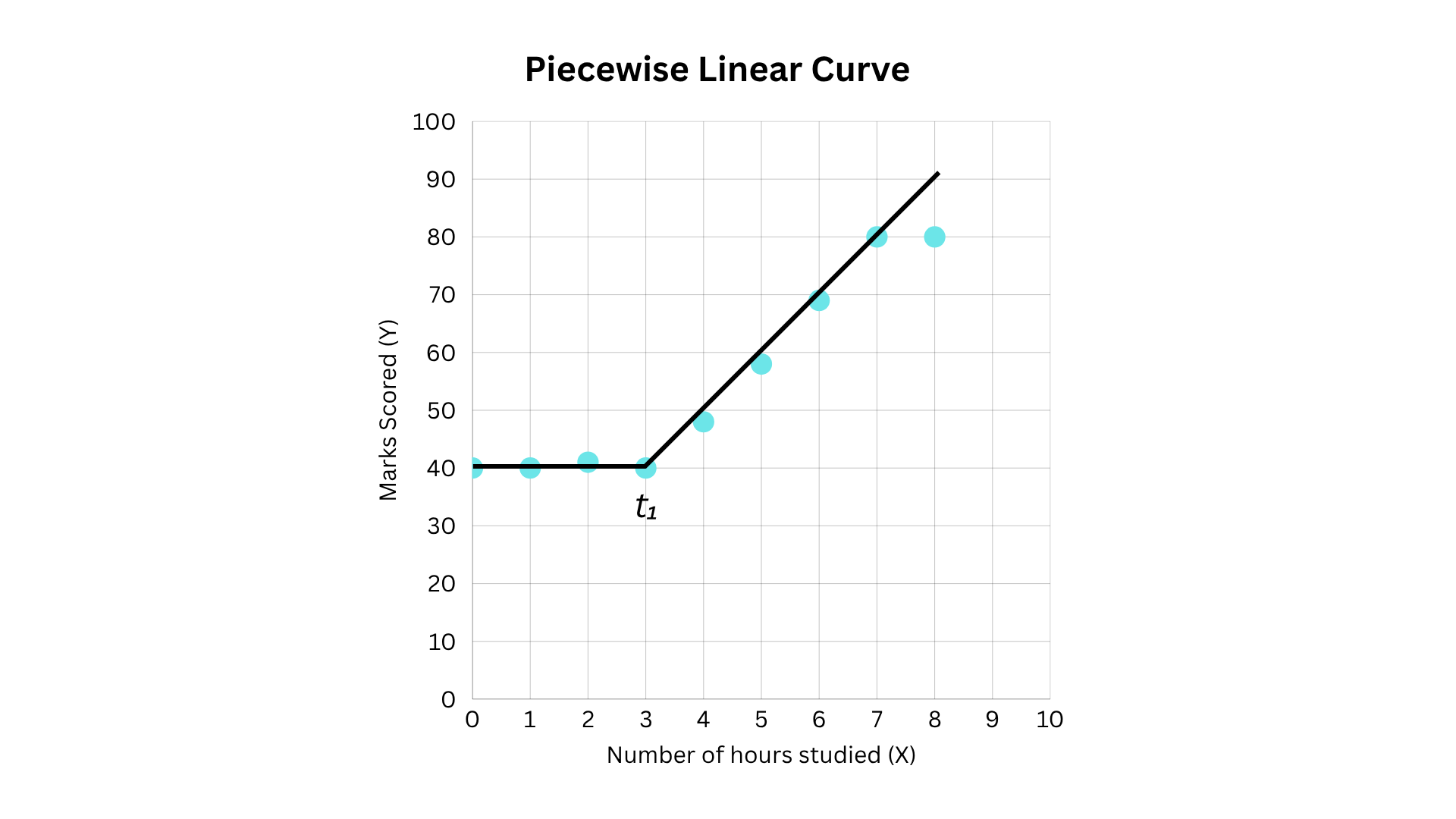
Individually, these may seem like straight line equations. But when put together, the overall relationship is no longer a straight line. When x crosses a certain value, the equation changes. This is called piecewise linear function. It's a function that's made up of different rules for different ranges of input.
This idea appears in one of the most widely used activation functions in neural networks: ReLU.
What is a ReLU Function?
ReLU stands for Rectified Linear Unit. Mathematically, it's this:
y = ReLU(x) = max(0,x)
It keeps positive inputs unchanged and turns negative inputs to zero.
Here too, the individual piece is linear but the overall function is non-linear. So, ReLU is a piecewise linear function that introduces non-linearity.
The graph below shows the ReLU function:
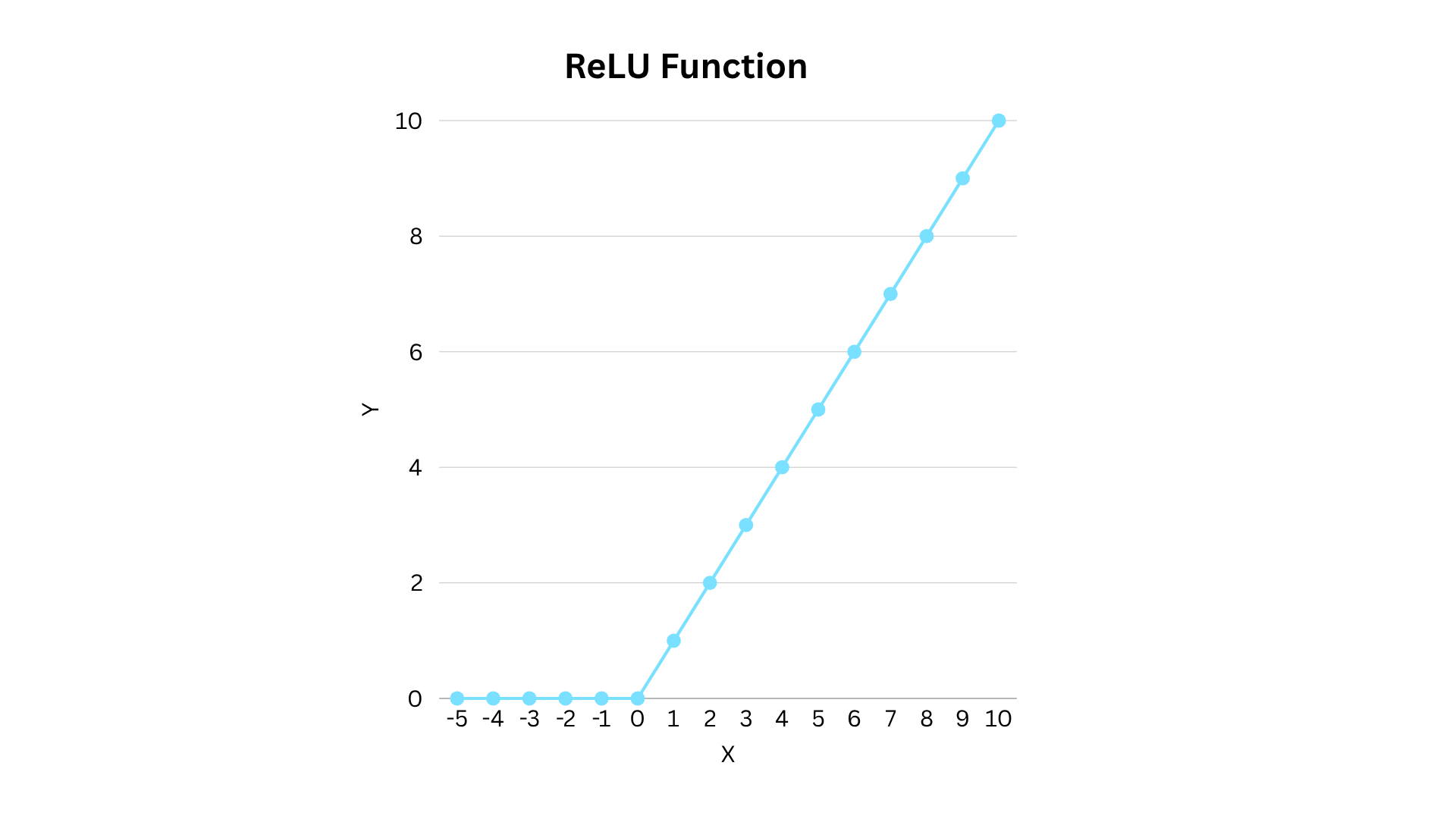
This simple change in behaviour allows a neuron to respond differently to different ranges of input, giving neural networks a way to move beyond a single straight-line relationship.
S-Shaped Curve
Now, a piecewise linear curve does the job but Ms. Poly sees that there's quite a sharp transition from one region to the other. She had also only considered two regions for simplicity, even though the distribution can be divided into three regions.
So, she draws a smooth curve roughly passing through all the points as shown below:
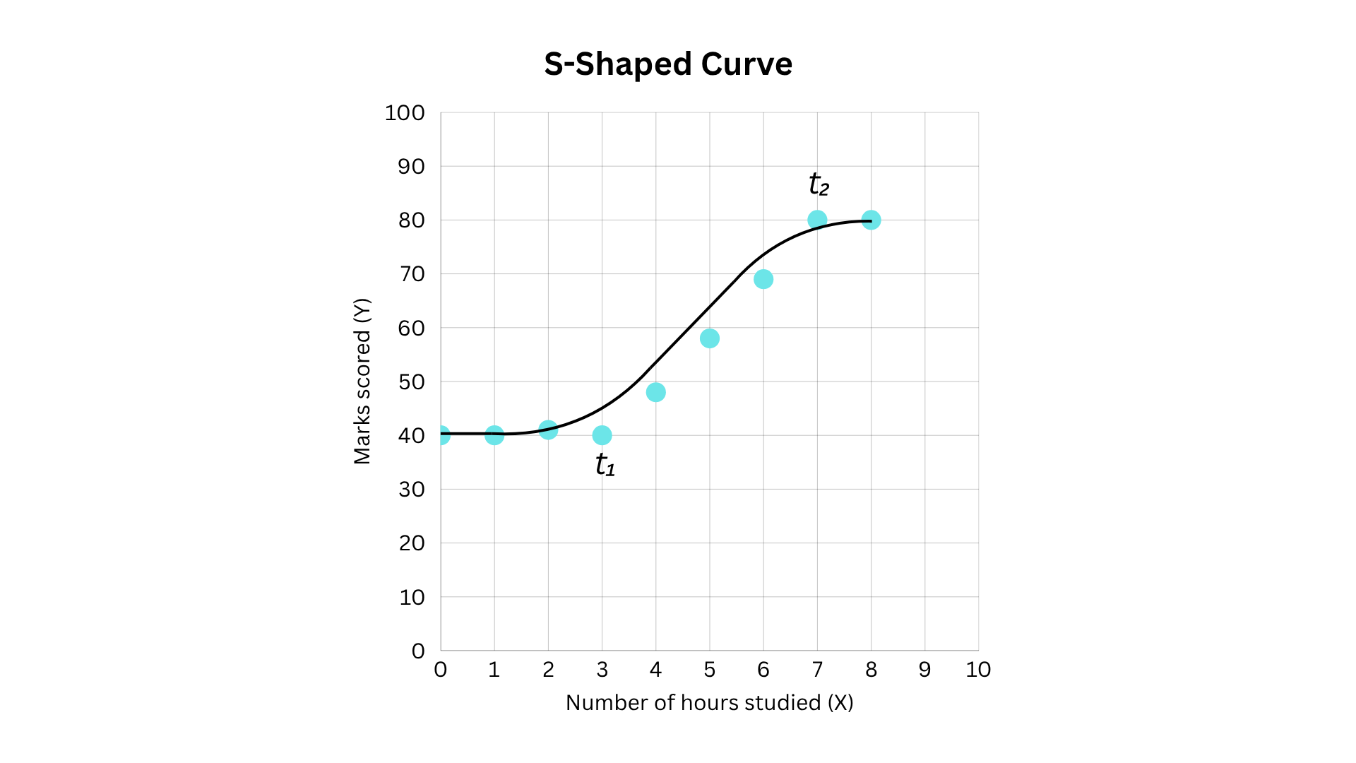
This shape shows that the marks remain almost the same when a student studies for up to t₁ number of hours. Then, an increase in hours of study from t₁ to t₂, increases the marks scored, so there's a slope. In the end at t₂, it flattens out again. This transition is gradual and continuous unlike the piecewise linear curve which changes directions using simple straight lines.
The curve that Ms Poly drew isn't some random pattern. It can be represented mathematically, too. One of the functions that produces this kind of shape is the sigmoid function.
What is a Sigmoid Function?
A sigmoid function is a mathematical formula that takes any real-valued input and maps it to values between 0 and 1. It slowly increases from values close to 0, rises quickly in the middle and gradually levels off at values close to 1.
y = σ(x) = 1 / (1 + exp(-x))
The graph below shows the sigmoid function:
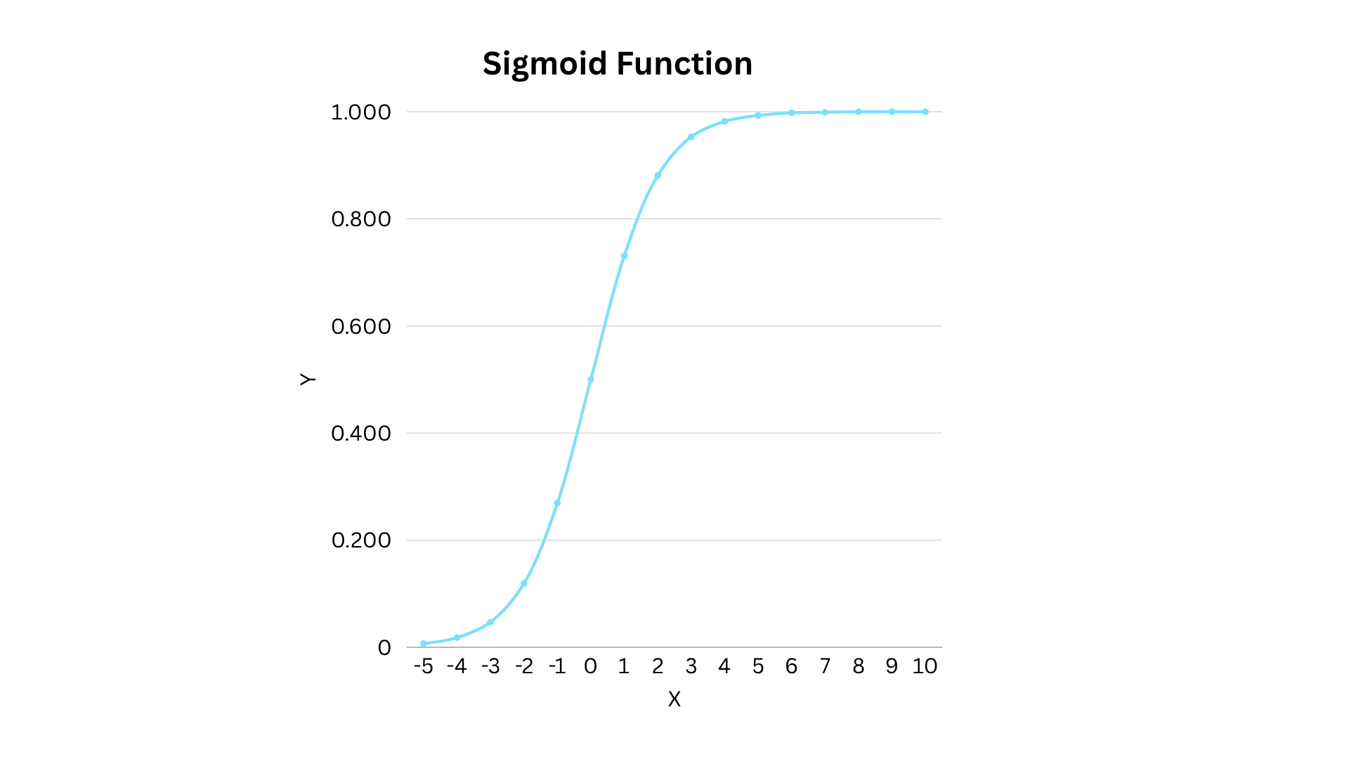
The sigmoid function is significant in neural networks because it introduces non-linearity while also restricting the output between 0 and 1. This makes it useful when the output needs to represent a probability such as the likelihood of a student passing an exam. A higher sigmoid output indicates a higher probability of the student passing, and vice versa.
Modeling a Deep Neural Network
Ms Poly should now combine the concepts of linear and non-linear equations to model a deep neural network. She has to take two separate approaches to ,
Predict the marks scored in the exam
Predict Pass/Fail in the exam
She uses two very simple untrained neural networks with manually chosen weights and biases for each. She is just trying it out to illustrate how calculations work. In reality she wouldn't choose the parameters herself. She would set up the network with weights and biases being learnt during training by repeatedly comparing the predicted values with the actual values and adjusting the parameters to minimise the error.
Predicting Marks Using ReLU
Step #1: Set up the network
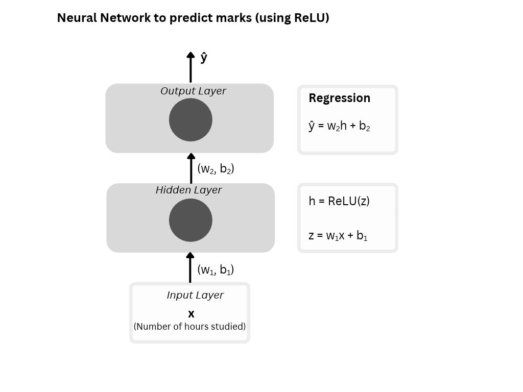
Ms Poly has the set up the deep neural network with simple equations in the following way:
Input Layer: The number of hours studied (x) is received here.
Hidden Layer: Linear transformation and ReLU is applied to the input.
z = w₁x + b₁, = x - 3      (w₁=1, b₁=-3)
h = ReLU(z) = max(0, z)
Output Layer: The marks scored is predicted after applying a linear transformation to the hidden layer's output(h).
ŷ = w₂h + b₂ = 10h + 40 (w₂=10, b₂=40)
Step #2: Calculate the Predicted Marks
Suppose she wants to calculate the marks scored by a student who studies for 5 hours. This is how she does it:
z = w₁x + b₁, = x - 3 = 5 - 3 = 2
h = ReLU(z) = max(0, z) = max(0, 2) = 2
Finally calculate the predicted marks:
ŷ = w₂h + b₂ = 10h + 40 = 10(2) + 40 = 60
The neural network predicts 60 marks whereas the actual marks in the dataset is 58.
Step #3: Compare Predictions with Actual Marks
After Ms Poly gets all the marks predicted by the neural network, she compares them with the actual data in the table below:
| Number of Hours Studied | Marks Scored | Predicted Marks |
|---|---|---|
| 0 | 40 | 40 |
| 1 | 40 | 40 |
| 2 | 41 | 40 |
| 3 | 40 | 40 |
| 4 | 48 | 50 |
| 5 | 58 | 60 |
| 6 | 69 | 70 |
| 7 | 80 | 80 |
| 8 | 80 | 90 |
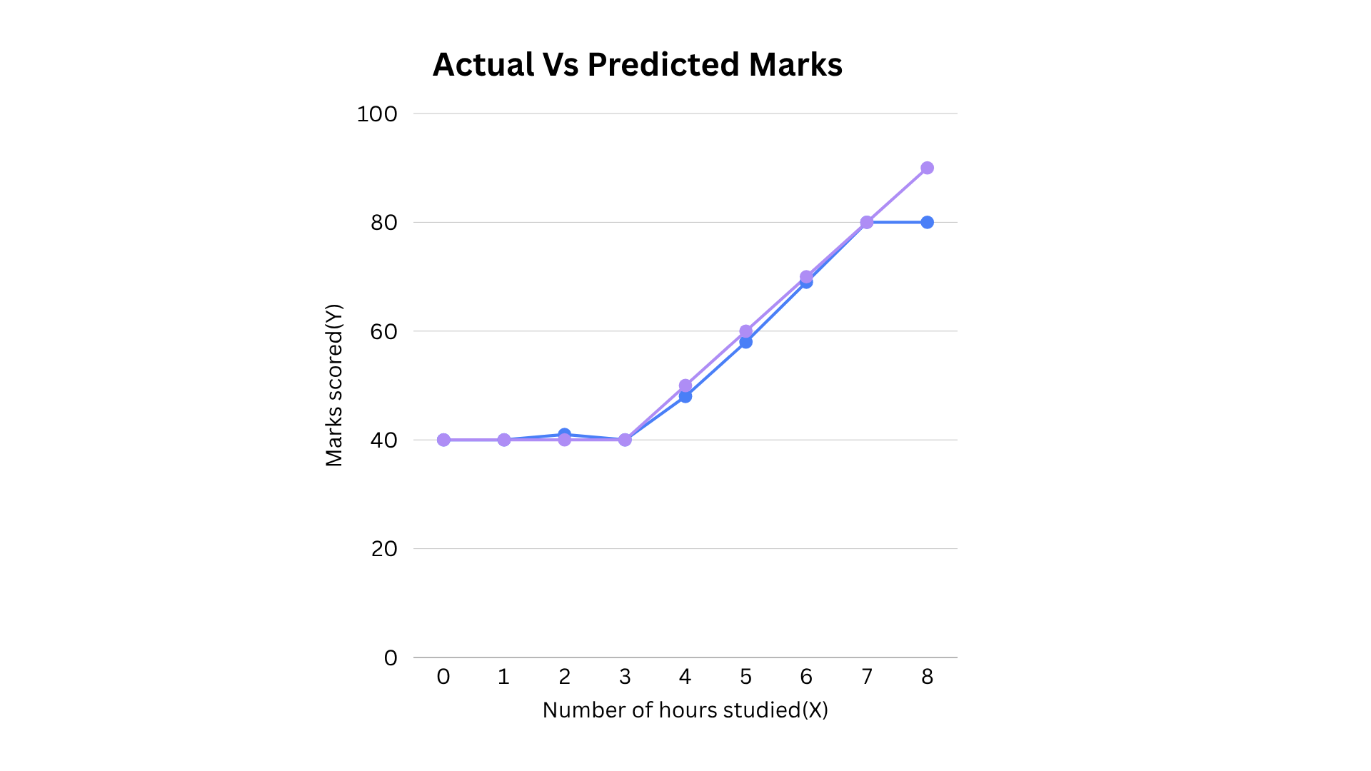
The actual and predicted marks don't match exactly, but they're close. The marks keep increasing and don't flatten out in the end because the value keeps increasing after the ReLU threshold.
Through this example Ms Poly has demonstrated how ReLU helps in modeling non-linear relationships in the data.
Predicting Pass/Fail Using ReLU and Sigmoid
Here Ms Poly will use a neural network to predict whether a student passes or fails in the final exam. She assumes a student needs to score a minimum of 50 marks to pass. This network will be used to predict the probability of passing the exam.
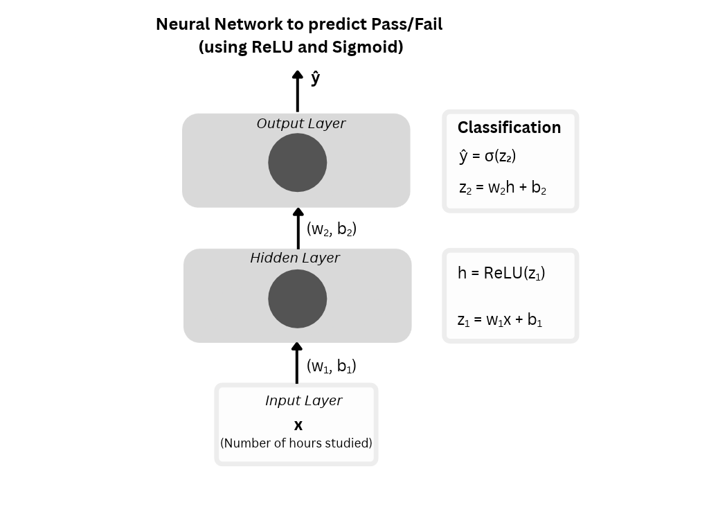
Step #1: Set Up the Network
Ms Poly has the set up the deep neural network with simple equations in the following way:
Input Layer: The number of hours studied (x) is received here.
Hidden Layer: Linear transformation and ReLU is applied to the input.
z₁ = w₁x + b₁, = x - 4      (w₁=1, b₁=-4)
h = ReLU(z₁) = max(0, z₁)
Output Layer: The pass/fail is predicted after applying sigmoid activation to the linear transformation of the hidden layer's output(h).
z₂ = w₂h + b₂ = 2h - 1      (w₂=2, b₂=-1)
p = σ(z₂) = 1 / (1 + exp(-z₂))
ŷ = Pass, if p >= 0.5
ŷ = Fail, if p < 0.5
Step #2: Calculate the Pass/Fail Prediction
Suppose she wants to predict the result for a student who studies for 3 hours. This is how she does it:
z₁ = w₁x + b₁, = x - 4 = 3 - 4 = -1
h = ReLU(z₁) = max(0, z₁) = max(0, -1) = 0
Predicting if the student passes/fails:
z₂ = w₂h + b₂ = 2h - 1 = 2(0) - 1 = -1
p = σ(z₂) = 1 / (1 + exp(-z₂)) = 1 / (1 + exp(-(-1))) ≈ 0.269
Since 0.269<0.5, the student's result is Fail.
Now for the result of a student who studies for 5 hours:
z₁ = w₁x + b₁, = x - 4 = 5 - 4 = 1
h = ReLU(z₁) = max(0, z₁) = max(0, 1) = 1
Predicting if the student passes/fails:
z₂ = w₂h + b₂ = 2h - 1 = 2(1) - 1 = 1
p = σ(z₂) = 1 / (1 + exp(-z₂)) = 1 / (1 + exp(-1)) ≈ 0.731
Since 0.731>0.5, the student's result is Pass.
Step #3: Compare Predictions with Actual Results
| Number of Hours Studied | Marks Scored | Actual Result | Predicted Score | Predicted Result |
|---|---|---|---|---|
| 0 | 40 | Fail | 0.269 | Fail |
| 1 | 40 | Fail | 0.269 | Fail |
| 2 | 41 | Fail | 0.269 | Fail |
| 3 | 40 | Fail | 0.269 | Fail |
| 4 | 48 | Fail | 0.269 | Fail |
| 5 | 58 | Pass | 0.731 | Pass |
| 6 | 69 | Pass | 0.953 | Pass |
| 7 | 80 | Pass | 0.993 | Pass |
| 8 | 80 | Pass | 0.999 | Pass |
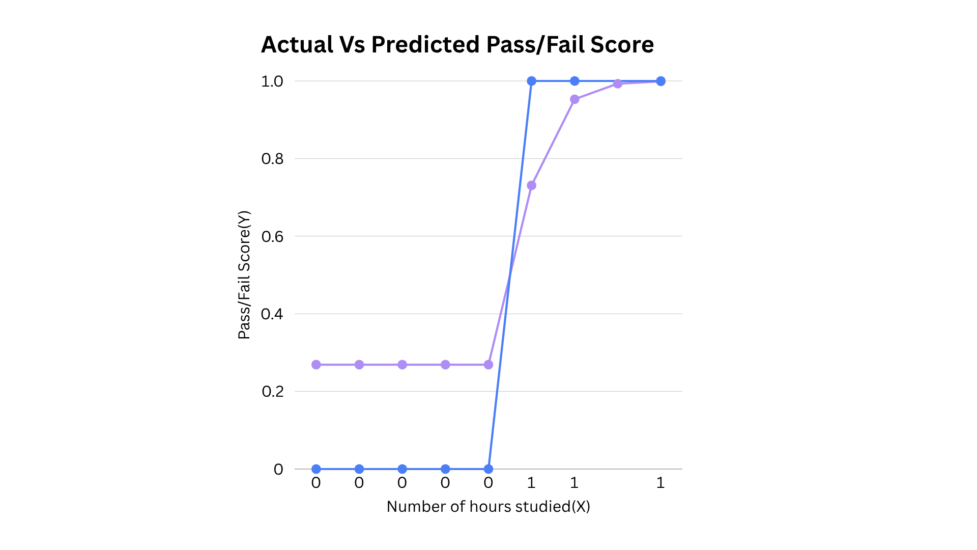
The network correctly classifies the result of all the students in this example. As the study hours increase beyond 4, the predicted score increases, making pass prediction more likely.
Through this example Ms Poly has demonstrated how ReLU and sigmoid work together. ReLU transforms the input in the hidden layer and sigmoid helps in converting the output to a score that can be used to make Pass/Fail prediction.
Final Thoughts
The simple examples shown above help us understand an important rule about neural networks: the relationship between the outputs and the inputs can behave differently across different parts of the input. They need to be captured in order to produce meaningful results from real-world data.
A straight line equation is enough when the relationship in data is simple and consistent. But real-life data isn't always that straightforward. By introducing non-linearity, neural networks can move beyond straight-line relationships and learn complex relationships hidden in data.


