

Searching is something people do every day. Whether they're word searching in documents and databases, or pattern matching in bioinformatics to detect anomalies in DNA, the applications for search are pretty much endless.
And these applications require a lot of computation. Imagine searching for a particular DNA sequence out of millions, or searching for a user in Google's database.
That's why we need an algorithm that runs very fast without consuming lots of memory. And that's what you'll learn about here.
In this tutorial, we will be diving deep into two famous search algorithms: Rabin-Karp's algorithm and the Knuth-Morris-Pratt algorithm. We'll also discuss their time and space complexity, which is equivalent to the time and space an algorithm consumes, depending on its input size. You will also learn about common data structures for searching.
A very basic knowledge of programming is required to follow along. We'll be using Python examples in this tutorial.
Table of Contents
- Data structures for bioinformatics and searching
- Naïve search algorithm
- Rabin-Karp's algorithm
- Knuth-Morris-Pratt algorithm
- Conclusion
Data Structures for Bioinformatics and Searching
Let's first discuss some data structures that you should know even if we weren't diving too deeply into the topic.
The Trie Data Structure
A trie is a tree-like data structure where each nodes stores a letter of an alphabet. You can structure the nodes in a certain way so that words and strings can be retrieved from the structure by traversing down a branch (path) of the tree.
Let's take the words ANA, AND, and BOT for example – their prefix tree or trie will look like this:
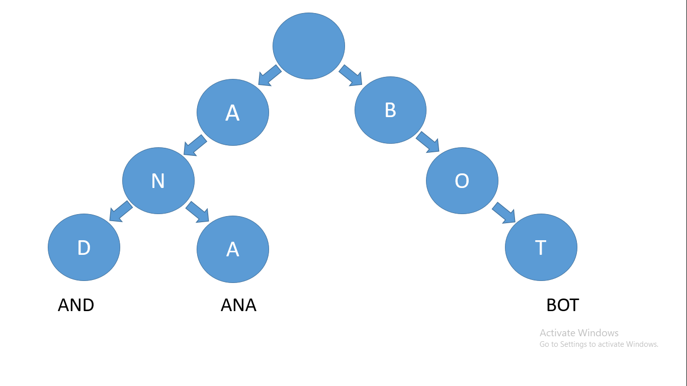 How a trie looks like
Tries are widely used for:
- Auto complete
- Spell Checkers
- Longest prefix matching
- Browser history
Suffix trees
Suffix trees are tree-based data structures, but instead of taking multiple words to build the tree we will be using the suffixes of a single world.
If we consider the string AABA, we will first add a $ sign to the end of the string. That $ will make string comparison easier. Now the string is AABA$.
We will consider all of it's suffixes and the tree will look like this:
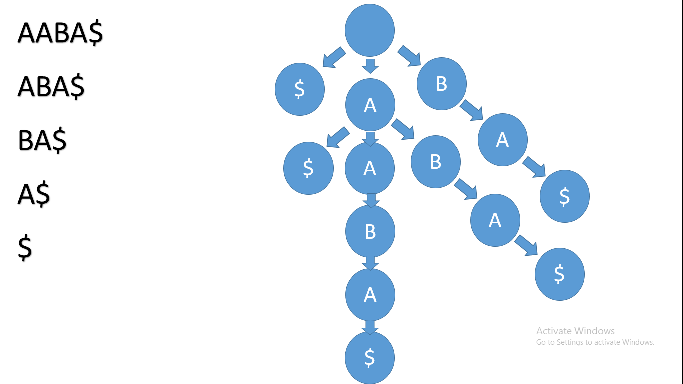 A suffix tree
Burrows Wheeler transform
Now we will discuss the burrows wheeler transform which is very useful data structure fort string compression.
This data structure is widely used in bioinformatics for a very specific reason. I want you to imagine a string representing a genome. It maybe very long, like 20 million characters.
But there is actually a way to store genomes efficiently. Imagine the string AAAAABBBAAA. This string has many repeats and we can actually compress this string to be something like this: A5B3A3. This is very useful for genomes as well which have many repeated characters.
Now let's take the string BANANA. We will first add a $ sign to the start of the string then compute all the cyclic rotations of $BANANA. Then will sort the cyclic rotations – and here is the importance of the dollar sign: that value, when sorting, is less than all alphabet values, so it will make sorting way easier.
After we sort the cyclic rotations, the string formed by the last characters of the sorted cyclic rotations is the burrows wheeler transform. It will look like this:
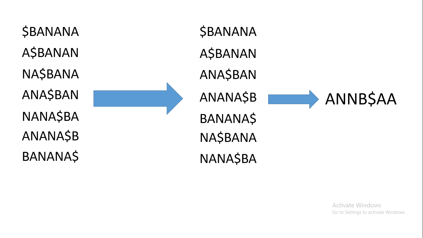 Burrows wheeler transform
Now as you can see, the burrows wheeler transform tends to have lots of repeats. You might also ask how to reverse the operation. To do that, look at the first characters of the sorted cyclic rotations. They are the same as the characters in the burrows wheeler transform but in sorted order.
So by sorting the burrows wheeler transform, we will get the first and the last letters and compute the original string.
Naïve Search Algorithm
Now let's look at a brute force solution for finding a pattern in a string. This approach is not optimal, as it runs with O(n*m) time complexity (where m is the length of the pattern and n is the length of the string).
We will consider two pointers, I and J. First we'll initialize I and J to be 0. Then we will run a while loop that will keep running while I is less than the length of the string.
Every time the loop runs we will compare the characters at the index I+J in the string and the character at the index J in the pattern. If they are equal, we will increment J, but of mpt. we will increment I and reset J to be 0. If j ever exceeds the length of the pattern, then there's a match.
The code for this will look like this:
def Find_Match(pattern,string):

  #initialise i and j
  i=0
  j=0

  while i<len(string):
   if string[i+j] == pattern[j]:
     j+=1
   if string[i] != pattern[j]:
     j=0
     i+=1
   #Let's say j is equal to the length of the pattern. Then to reach the first match index we can go back a number of steps equal to the length of the pattern.
   if j==len(pattern):
    return i-j

  #Incase there is no match
  return -1
Rabin-Karp's Algorithm
The problem with the naïve approach is that it runs in O(n**2) time complexity which is horrible when it comes to large inputs like genomes. This means we need something better.
Comparing two strings is linear time, because we need to compare each character for each index. But what if we don't need to do that – what if we transformed the strings into numbers?
Here is the main idea of this algorithm. Let's say there is a function that returns a number associated with each string in the alphabet. We will use the ASCII value of the strings for that.
And then to transform a string into a number we will compute the sum of the ASCII values of all its characters. This a simple hashing function:
def hash(string):
 count=0
 # in python ord return the ascii value of a character
 for i in string:
  count+=ord(i)

 return count
Now let's say we want to find an in banana. Then we will first compare hash(an) to hash(ba) then to hash(an) and so on till we reach the end of the string. When the hash values match, we can then compare the pattern and the substring because hash(na) and hash(an) are equal so we need an extra check.
You might be thinking this is silly – why do we need to do all of this? Computing the hash function needs to iterate over the string so we didn't achieve any better time complexity. And you're completely right.
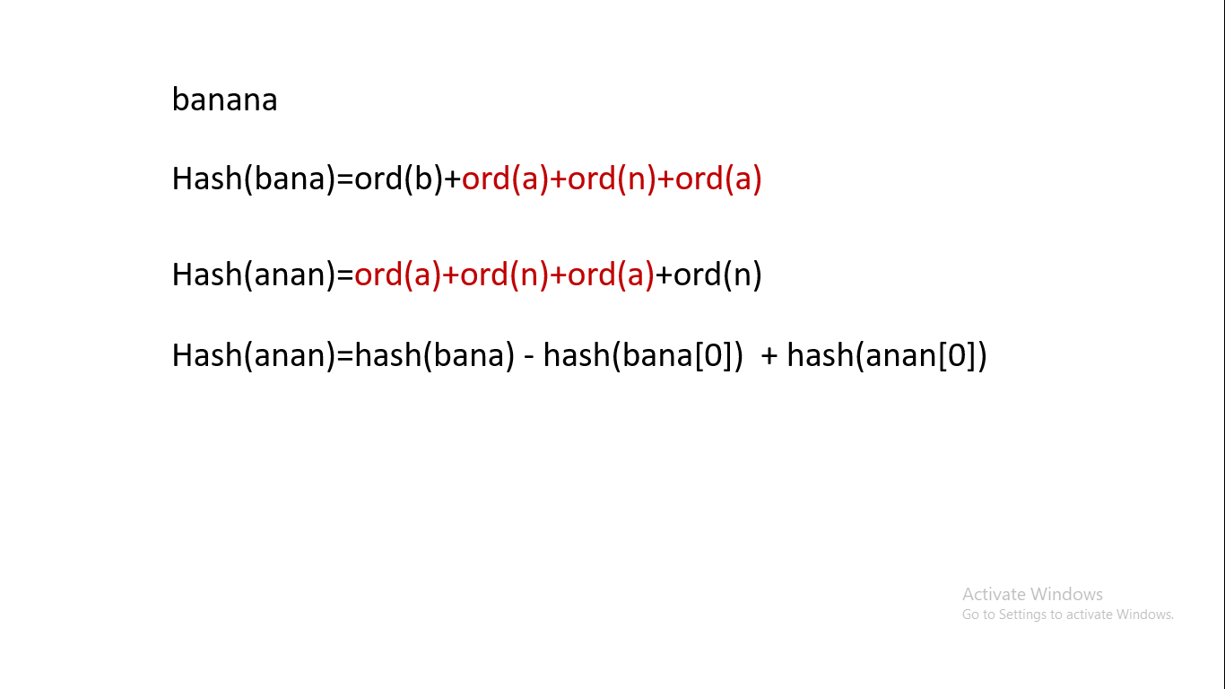
But what if we can compute the hash value of a substring from its previous substring? The difference is in the starting and ending characters – and that's called a rolling hash. That's what makes this algorithm run at O(n*m) worst case and O(n+m) average case: because of collisions.
For example, hash(na) is equal to hash(an), so here we need to compare na and an. The hash function I showed you is a very simple one. The better the hash function, the fewer collisions we will have. But I don't want to make this too fancy, so I will be using this hash function.
 rolling hash
def Rabin_Karp(string, pattern):
 #compute the hash value of the pattern
 hashed_pattern=hash(pattern)

 #compute the hash value of the first substring with length equal to the length of the pattern

 first_hash=hash(string[0:len(pattern)])

 for i in range(len(string)-len(pattern)+1):
  if i !=0:
   first_hash-= hash(string[i-1])
   first_hash+= hash(string[i+len(pattern)-1])

  if hashed_pattern == first_hash:
   #second check
   if pattern == string[i:len(pattern)]:
    return i

 #in case no matches are found
 return -1
Knuth-Morris-Pratt Algorithm
Now we will discuss the last algorithm for today. This one is very complicated but I will try to make it as simple as possible.
The idea behind this algorithm is that the naïve approach is great unless the string and the pattern have many repeats – like for example searching for AAAB in AAAXAAA. In this case do we really need to reset the j pointer to 0 after the first mismatch? Actually no we don't, and I will show you why.
When we analyze this pattern, we can see that it's quite special. Let's say we started at i=0 and we reached j=3. Then the next iteration we got a mismatch.
We don't really need to reset j, since for this given pattern we have the two first characters equal to the second and third characters. And since j already was 3, then the first 3 characters in the string are equal the first three characters in the pattern. And the second and third characters in the string are equal to the first and second characters in the pattern. So we can skip two positions by resetting j to 2 instead of 0.
Now you might ask how we'll know the value of j after the mismatch. Well, the answer depends on the pattern. For example abac if we got a mismatch when we reached j=3 (when we reached c) and since ab is equal to ba, we can actually skip b for the next iteration.
As you can see this works when we have a common suffix and prefix in a substring of a pattern, so we need to preprocess the string. And for each index of that substring, we can compute the number of skips and store it in an array known as the longest suffix prefix array.
Now we'll write the function for computing the LSP array. But first I will explain what I will be doing:
- the first element in the array is always 0
- we will create an array LSP with the same length as the pattern
- we will have twp pointers i and prevlps. i is an iteration variable initially set to 1, since the first element in the array is always 0. prevlps keeps track of the previous longest prefix suffix.
- we will run a while loop which will keep running while i is less then the length of the pattern. It will compare pattern[i] and pattern[prevLps]. If they match, we will set LCP[i] to prevlps +1, and we'll increment i and prevlps by 1.
- if they don't match and prevlps was 0 already, we will set LCP[i] to 0 and increment i.
- if prevlps was not 0, we will set prevlps to LCP[prevlcp-1].
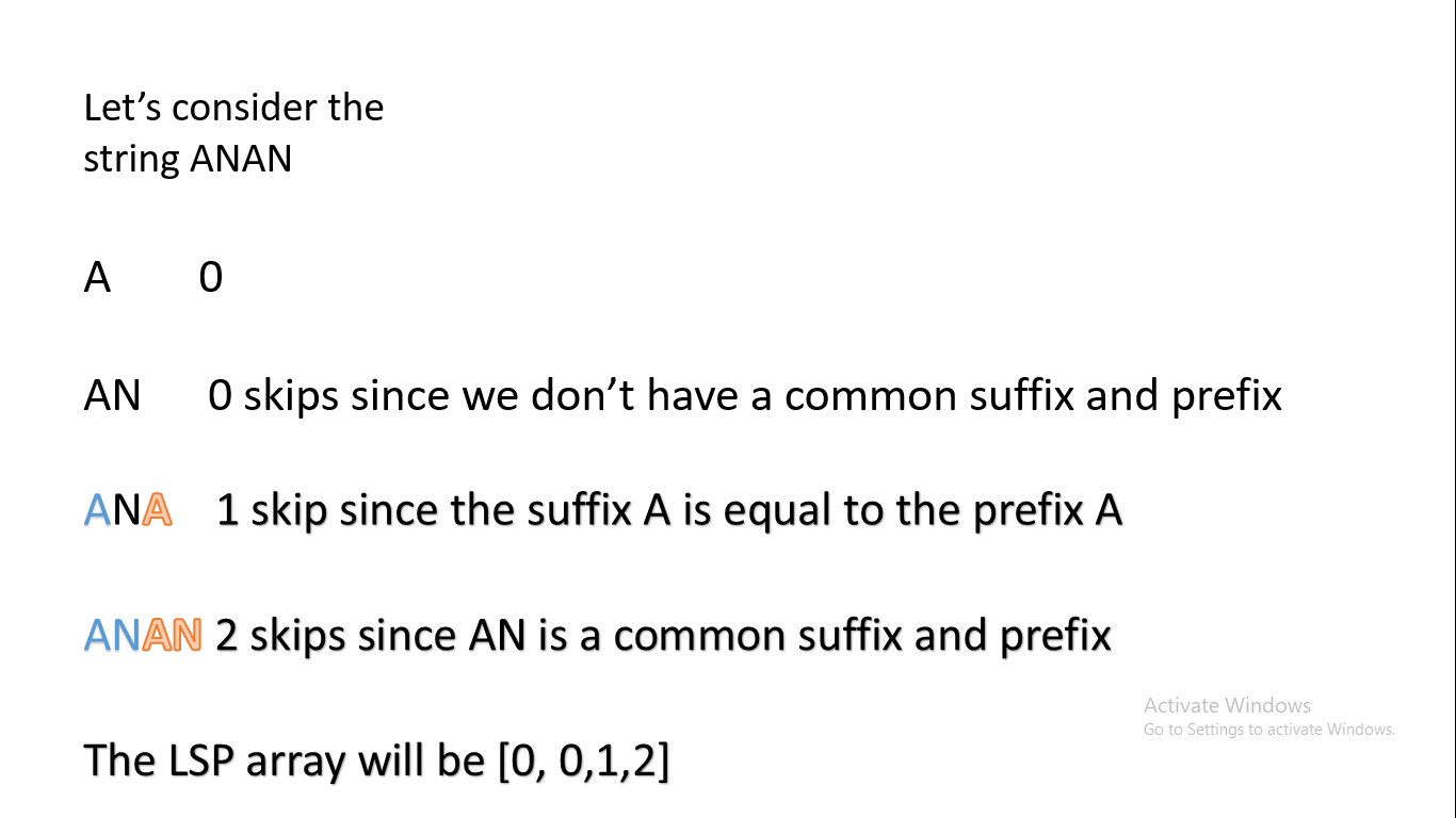
Let's take an example using the string ANAN. First i was 1 and prevlps was 0. The first iteration happens, and A is not equal n and prevlps is 0 – so the LCP is now [0,0,0,0].
Now for the second iteration we will compare pattern[prevlps] which is A and A which evaluates to true. So now i is 3, prevlps is 1, and LCP is [0,0,1,0].
And finally, in the final iteration we will compare N and N. The same thing happens as in the past iteration, and LCP is [0,0,1,2].
The code for LCP is the following:
def LCP(pattern):
 LCP_array=[0]* len(pattern)

 i=1
 prevlcp=0

 while i<len(pattern):
  if pattern[i]==pattern[prevlcp]:
   LCP_array[i]=prevlcp+1
   i+=1
   prevlcp+=1

  elif prevlcp == 0:
   LCP_array[i]=0

  else:
   prevlcp=LCP_array[prevlcp-1]

 return LCP_array
Now since we have the LCP array we can run the KMP algorithm. It's similar to the naïve algorithm but with some improvements. It will look like this:
def KMP(pattern,string):

  LCP_array=LCP(pattern)

  #initialise i and j
  i=0
  j=0

  while i<len(string):
   if string[i+j] == pattern[j]:
     j+=1
   if string[i] != pattern[j]:
     #The line that changed
     j=LCP_array[j-1]
     i+=1
   #Let's say j is equal to the length of the pattern. Then to reach the first match index we can go back a number of steps equal to tje length of the pattern.
   if j==len(pattern):
    return i-j

  #In case there is no match
  return -1
This algorithm runs with O(n+m) time complexity which is great – but it's little bit complicated. If you noticed, almost nothing changed (just in computing the LCP and a single line changed). This single line is what makes the algorithm so efficient.
Conclusion
In the end I hope you learned something new from this article. We learned about data structures for searching as well as some famous algorithms for searching.
This tutorial was the result of two weeks of research. There are a lot of things that I wanted to cover but I wanted to keep this manageable.
If you found this useful and want to get more awesome content, follow me on LinkedIn. It will help a lot.