

Ever wondered how algorithms predict future house prices, stock market trends, or even your next movie preference? The answer lies in a fundamental yet powerful tool called linear regression.
Don't be fooled by its seemingly simple equation – this article will unveil its magic, empowering you to build and understand these models, whether you're a machine learning newcomer or a seasoned expert who needs a refresher.
In this article you will get crystal clear explanations, hands-on guidance, and real world applications where you will witness the power of linear regression in action.
So, buckle up and get ready to conquer the straight and narrow path of linear regression! By the end of this comprehensive guide, you'll be equipped to confidently build, interpret, and leverage these models for your own data-driven endeavors.
Table of Contents
Prerequisites
Before we begin, make sure you have the following installed:
Python (3.x recommended)
Jupyter Notebook : this is optional but recommended for an interactive environment and also for trial and error (beginners will benefit the most from this)
Required libraries: pandas, NumPy, Matplotlib, seaborn, scikit-learn
You can install these libraries using pip install in the command line:
pip install pandas
pip install matplotlib
pip install numpy
pip installseaborn
pip install scikit-learn
What is Linear Regression?
In simple terms, Linear Regression harnesses the power of straight lines.
Imagine you are a realtor trying to predict the price of a house. You might consider various factors like its size, location, age and number of bedrooms.
Linear regression comes in as a powerful tool to analyze these factors and unveil the underlying relationships. It is a powerful statistical technique that allows us to examine the relationship between one or more “independent” variables and a “dependent” variable.
In a house price dataset, the independent variables are columns used to predict, such as the “Area”, “Bedrooms”, “Age”, and “Location”. The Dependent variable will be the “Price” column – the feature to be predicted.
Linear regression is the simplest form of regression, assuming a linear (straight line) relationship between the input and the output variable. The equation for simple linear regression can be expressed as y = mx + b, where, y is the dependent variable, x is the independent variable, m is the slope, and b is the intercept.
This creates a best fit line, but do not worry too much about the underlying math. However, it is important as you go further in your machine learning journey.
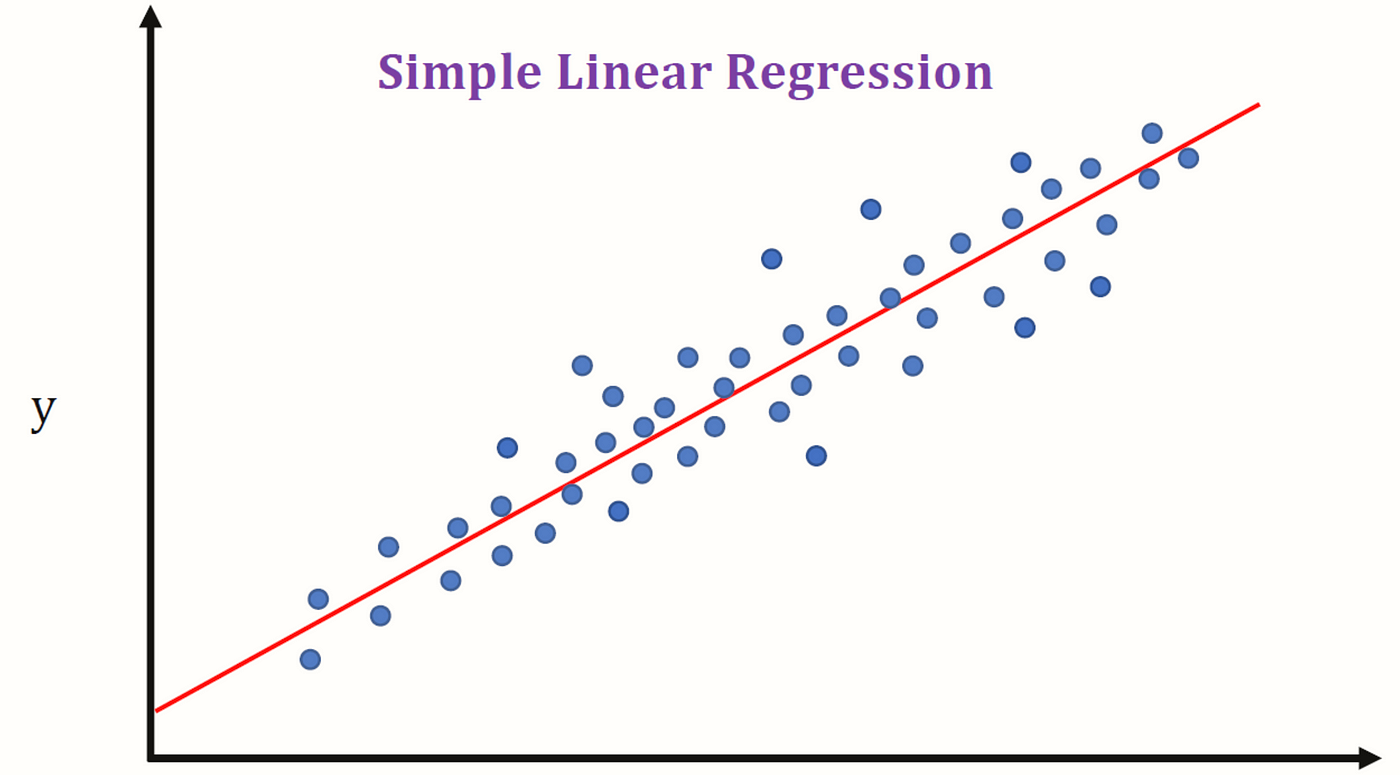
Simple linear regression graph
Why is Linear Regression Valuable?
Interpretability: Unlike some complex models, linear regression provides clear insights into how each feature influences the target variable. You can easily see which features have the strongest impact and how they contribute to the overall prediction.
Baseline for complex models: When dealing with more intricate problems, data scientists often start with linear regression as a baseline model. This simple model serves as a reference point to compare the performance of more complex algorithms. If a complex model doesn't offer significantly better results than linear regression, it might be unnecessarily overfitting the data.
Ease of implementation: Compared to other machine learning algorithms, linear regression is relatively easy to implement and understand. This makes it a great starting point for beginners venturing into the world of machine learning.
Remember, linear regression might not be the ultimate solution for every problem, but it offers a powerful foundation for understanding data, building predictions, and setting the stage for exploring more complex models.
Let us dive deeper into the mechanics of building and interpreting linear regression models.
Linear Regression Key Concepts
Ready to dive deeper into the mechanics of linear regression? Don't worry, even without a PhD in math, we can unlock its secrets together without getting bogged down in the complicated terms.
What happens when your create a Linear Regression Model?
Find the best fit line: Lines are drawn across a graph, with features on one axis and prices on the other. The line we're looking for is the one that
best fitsthe dots representing real houses, minimizing the overalldifferencebetween predicted and actual prices.Minimize the error: Think of the line as a
balancing act. The line's slope and position is adjusted until the total distance between the line and the data points is as small as possible (Minimized Cost Function). This minimized distance reflects the best possible prediction for new houses based on their features.Coefficients: Each feature in the model gets a
weight(Coefficients), like a specific amount of an ingredient in a recipe. By adjusting these weights, we change how much each feature contributes to the predicted price. A higher weight for size, for example, means that larger houses tend to have a stronger influence on the predicted price.
So, what do we get out of this?
Once we have the best-fit line, the model can predict the price of new houses based on their features. But it's not just about the numbers – the weights tell a story.
They reveal how much, on average, each feature changes the predicted price. A positive weight for bedrooms means that, generally, houses with more bedrooms are predicted to be more expensive.
Assumptions and Limitations
Linear regression assumes things are roughly straightforward, like the relationship between size and price. If things are more complex, it might not be the best tool.
But it's a great starting point because it's easy to understand and interpret, making it a valuable tool to explore the world of data prediction.
However, you do not have to worry about finding the best fit line manually. The algorithm picks the best fit line when creating the model.
In the next section, you will learn how to build your very first House Price Prediction model.
How to Build Your First Model
How to import libraries and load data
If you are new to machine learning models, the libraries are imported as abbreviations for the sole purpose of writing shorter code:
import pandas as pd
import numpy as np
import matplotlib.pyplot as plt
import seaborn as sns
from sklearn.model_selection import train_test_split
from sklearn.linear_model import LinearRegression
from sklearn.metrics import mean_squared_error

# Load your dataset (replace 'your_dataset.csv' with your file)
df = pd.read_csv('your_dataset.csv')

# Display the first few rows of the dataset
df.head()
The dataset is loaded using pandas’ read_csv function and then the first five rows are displayed using df.head().
Exploratory Data Analysis (EDA)
Data from different sources are usually messy, scattered, they contain missing values, and are sometimes unstructured.
Before building a regression model, it's crucial to understand the data, and clean and optimize it for the best result. For an in-depth explanation check out this article on data cleaning and preprocessing.
Let's go over the steps you should take before building your model.
Check for missing values
Machine learning models cannot function when there are missing values in the dataset:
df.isnull().sum()
This will give you a list of columns that have null values and the rows themselves. There are different ways to deal with this such as:
Deleting all rows with null values.
Using the mean or median of the column to fill in the missing values for numerical data.
Filling the missing values with the most occurring data for qualitative data.
Explore the correlation between variables
sns.heatmap(df.corr(), annot=True, cmap='coolwarm')
plt.show()
This code will show the relationships between the columns of independent / variables / features, and dependent/ target variables.
It will also show which columns or features determine the outcome of the target variable more than others.
Visualize the relationship between independent and dependent variables
Scatter plots can show how well your predicted prices align with actual values. Residual plots help visualize any patterns in the errors, revealing potential issues.
sns.scatterplot(x='Independent Variable', y='Dependent Variable', data=df)
plt.show()
This scatter plot shows the relationship between independent and dependent variables and a straight line is drawn to show the relationship
Data preprocessing
This is a crucial step as the quality of data that is used to train the model also determines the accuracy and efficiency of the model.
Here, the data set is first separated into X (independent variable(s)/ features) and Y (dependent variable/ Target):
# Handle missing values if necessary
df.dropna(inplace=True)

# Split the data into features (X) and target variable (y)
X = df[['Independent Variable']]
y = df['Dependent Variable']

# Split the data into training and testing sets (e.g., 80% training, 20% testing)
X_train, X_test, y_train, y_test = train_test_split(X, y, test_size=0.2, random_state=42)
We handle the missing values by dropping columns with missing/ null values and split the dataset into training and testing in a 80:20 ratio.
Building the Regression Model
Finally , it is time to create and train our linear regression model.
We create a model by calling an instance of the model into a variable as shown below and train the model by fitting the training dataset into the model.
# Create a linear regression model
model = LinearRegression()

# Train the model
model.fit(X_train, y_train)
How to make Predictions
The trained model is used to make predictions on the test set. Predictions can be made on the entire feature column as shown below or each column can be predicted individually.
# Make predictions
y_predn = model.predict(X_test)
How to evaluate the Model
Evaluating the model's performance is an important step to determine the accuracy of the model and reusability. We can check using metrics such as:
“R-squared”: This tells you how well the model explains the variation in house prices. A higher value (closer to 1) indicates a better fit.
Mean Squared Error (MSE): This measures the average difference between predicted and actual prices. Lower is better.
Precision score.
# Evaluate the model
mse = mean_squared_error(y_test, y_pred)
print(f'Mean Squared Error: {mse}')

# Using precision score
model.score(X_test, Y_test)
How to visualize the results
Visualize the regression line and actual vs. predicted values:
# Plot the regression line
plt.scatter(X_test, y_test, color='gray')
plt.plot(X_test, y_pred, color='red', linewidth=2)
plt.xlabel('Independent Variable')
plt.ylabel('Dependent Variable')
plt.show()
Let's consider a different scenario where you want to flex your muscles and predict a student's score (y) based on the number of hours they studied (x). The linear regression model might look like this:
import numpy as np
from sklearn.linear_model import LinearRegression

# Sample data
hours_studied = np.array([2, 4, 6, 8, 10])
scores = np.array([60, 80, 90, 100, 95])

# Reshape the data
hours_studied = hours_studied.reshape(-1, 1)

# Create a linear regression model
model = LinearRegression()

# Fit the model
model.fit(hours_studied, scores)

# Make predictions
predicted_scores = model.predict(hours_studied)

the model model.fit(hours_studied, scores) # Make predictions predicted_scores = model.predict(hours_studied)
Advanced Linear Regression Techniques
You've conquered the basics of linear regression, but the journey continues!
Let's explore advanced techniques to unlock even more power and fine-tune your models.
Taming overfitting – Regularization
Imagine a cake smothered in frosting – impressive, but impractical.
Similarly, a model with too many features can "overfit" the training data, losing its ability to generalize. Regularization techniques act like seasoning, preventing this culinary catastrophe:
L1 (Lasso): Shrinks some coefficients to zero, effectively removing unimportant features.
L2 (Ridge): Shrinks all coefficients, preventing them from becoming too large.
These techniques penalize complex models, pushing them towards simpler solutions that generalize better to new data.
Feature engineering – Unearthing hidden gems
Not all features are created equal. Some might be redundant, while others hide valuable relationships. Feature engineering involves:
Selection: Identifying the most informative features using correlation analysis or statistical tests.
Transformation: Creating new features by combining existing ones (for example, multiplying square footage and bedrooms for total living area). This allows you to capture non-linear relationships beyond the linear model's capabilities.
By carefully selecting and transforming features, you can significantly boost your model's performance.
Categorical quandaries – Encoding and beyond
The world isn't always black and white. What about features like "city" or "property type"? These categorical variables require special handling:
One-hot encoding: Creates separate binary features for each category, allowing the model to learn their individual impact.
Polynomial features: Creates new features by interacting categories (for example, "city * property type"), capturing complex relationships.
Understanding how to handle categorical features unlocks valuable insights from your data. Check out this article for a deep dive on how to handle categorical features.
Model Selection – How to choose Your Champion
With this arsenal of techniques, you might have multiple models. How do you pick the best one? Consider:
Complexity: Simpler models are generally preferred, as they are less prone to overfitting.
Performance: Metrics like R-squared and cross-validation help compare models objectively.
Finding the right balance between complexity and performance is crucial for building effective and generalizable models.
Remember! Mastering linear regression is an ongoing journey. Experiment, explore these advanced techniques, and don't be afraid to get creative! With practice and curiosity, you'll unlock the true potential of this powerful tool and extract valuable insights from your data.
For further exploration check out the documentation:
Conclusion
This exploration of linear regression has equipped you with a robust understanding of its core concepts, model building process, and limitations.
Remember, this is merely the foundation. As you venture deeper, you'll encounter advanced techniques like regularization, feature engineering, and handling categorical features, unlocking even greater predictive power.
Embrace the spirit of exploration. Experiment, delve into the resources provided, and remember that mastering linear regression is an ongoing journey. Each challenge overcome, each model built, strengthens your ability to extract valuable insights from data.
So, continue learning, keep building, and unlock the true potential of this powerful tool.
If you found this helpful connect with me on LinkedIn.