
By Siddhesh Jadhav
This article is a step by step guide that'll help you interpret your machine learning model's predictions using LIME. Even when your model achieves close to 100% accuracy, there is always one question that runs in your mind: should we trust it?
Consider a situation at a doctor's office – would a doctor trust a computer if it just showed a diagnosis without giving any valid reason behind it?
Any model which fails to explain the reason behind its output is considered a black box. And trusting such a model is not the right approach.
Let's say we're given a model which predicts whether an animal is a dog or cat and has 100% accuracy. But what if it makes that prediction based on the background of the image? Would you trust that model?

As you can see in the above figure, the green color represents the features it took to identify the image as a cat, and the red indicates the features it took to represent it as a dog.
If our model provides such a valid reason for its prediction, it builds our trust for that model. Similarly for the doctor situation, if the model can tell which features were important in its prediction and to which symptoms it gave more weight, it is easier for the doctor to trust that model.
But it is that simple to interpret any model? Luckily yes. Marco Tulio Ribeiro, Sameer Singh, and Carlos Guestrin came out with a paper called "Why Should I Trust You?": Explaining the Predictions of Any Classifier in 2016.
In it, they proposed their technique LIME. The basic approach of this technique was to easily interpret any model by learning it locally around its prediction.
They wrote this paper to understand the explanations behind any model's prediction. So whenever you need to choose a model, you can use the insights from LIME.
 Explaining individual predictions using LIME source
In the above diagram, the model predicts that a patient has the flu, and LIME highlights the symptoms in the patient's history that led to the prediction.
Sneeze and headache contribute to the "flu" prediction, while "no fatigue" is evidence against it. With this information, a doctor can make an informed decision about whether to trust the model's prediction.
So, what exactly is LIME?
LIME is model-agnostic, meaning that it can be applied to any machine learning model. The goal of LIME is to identify an interpretable model over the interpretable representation that is locally faithful to the classifier.
- Definition from official paper (link)
To understand this, we need to understand the meaning of the acronym LIME.
Local: Refers to how we get these explanations. LIME approximates the black box model locally in the neighborhood of predictions.
Interpretable: The explanations provided by LIME are simple enough for humans to understand.
Model-agnostic: LIME treats the model as a blackbox, and so it works for any model.
Explanations: The justifications given for the actions performed by the model.
LIME provides local model interpretability. It modifies a single data sample by tweaking the feature values and observing the resulting impact on the output.
With LIME, we cane explain why the RandomForestClassifier thinks what it does before giving a prediction.
Let's look at some code
We'll start by using the RandomForestClassifier model to work on the "Did it rain in Seattle" dataset. The data is available here.
First we will import our base libraries:
import numpy as np
import pandas as pd
import matplotlib.pyplot as plt
%matplotlib inline
In order to avoid future warnings in our code, we will add this to our code at the start of our script:
import warnings
warnings.filterwarnings('ignore')
We then import a few sklearn libraries for splitting the dataset and for defining the metrics. The RandomForestClassifier will also be imported from the same library.
from sklearn.model_selection import train_test_split
from sklearn.metrics import accuracy_score
from sklearn.ensemble import RandomForestClassifier
Since we have all our required libraries, we will read our data:
df = pd.read_csv('seattleWeather_1948-2017.csv')
df.head()

So the data consists of 4 feature columns and a target column, i.e. RAIN. Our task is to predict if there was RAIN in Seattle.
df.shape
(25551, 5)
Our data consists of 25,551 rows which is enough for our model to train.
We will check for missing values, if any:
df.isnull().sum()
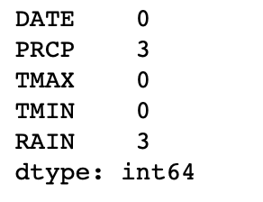
Since our main focus is interpreting the model's prediction, we will discard the missing value rows directly. For simplicity's sake we will remove the DATE column as well.
df.dropna(inplace=True)
df.pop('DATE')
We will now encode our target column:
df.RAIN.replace({True:1,False:0},inplace=True)
df.head()

This is how our data looks in the end.
target = df.pop('RAIN')
x_train , x_test , y_train , y_test = train_test_split(df, target, train_size=0.75)
We have now split the data into train and test sets with train equal to 75% of the original data.
We will now create our model with default parameters:
rfc = RandomForestClassifier()
And fit the model to the training samples:
rfc.fit(x_train,y_train)

accuracy_score(y_test,rfc.predict(x_test))
1.0
The model has achieved 100% accuracy. But now let's interpret the model so we can trust it.
LIME
First, we need to discuss a bit of theory before we go on.
LIME creates new data which includes permuted samples and its respective predictions.
On this, LIME trains a local model which is weighted by proximity of sample instances. This model can be any basic model, namely a Decision tree.
This model must have similar local predictions as that of the existing model. This accuracy is called local fidelity.
import lime
from lime import lime_tabular
Now that we have imported the required packages, we need to perform our interpretation.
Here's the recipe for training local surrogate models:
- Select the model for which you want to get the explanation of its prediction
- Train this model and get its prediction for the test values
- For LIME, we weight the new samples with respect to their proximity to the model
- Create a local model on the dataset
- Finally we explain the prediction by interpreting the local model
Define a LimeTableExplainer model. Parameters of this model are Training sample, Feature names, and class names:
explainer = lime_tabular.LimeTabularExplainer(x_train.values,feature_names=['PRCP','TMAX','TMIN'],class_names=['False','True'],discretize_continuous=True)
We need to pass training samples, the training column names, and the target class names that are expected.
We then call the explain_instance() function of the explainer we created.
We will be using the following parameters of this function - test sample, predict function of model, number of features, and top labels to consider:
i = np.random.randint(0,x_test.shape[0])
exp = explainer.explain_instance(x_test.iloc[i],rfc.predict_proba,num_features=x_train.shape[1],top_labels=None)
In order to display the explanation in the notebook, the following code is required.
exp.show_in_notebook()

Let's decrypt the output.
The top left diagram indicates the predicted output with probability.
The model's output is False with 100% probability.
The top right diagram indicates the conditions required to fall for each category with their weights.
Since the condition for PRCP variables for predicting the target as False is PRCP ≤0.00 and it has 0.96 weight.
The Bottom right diagram indicates our test values. Since the PRCP values satisfy for a False condition, you can see the blue color as the background for this.
To display the explanation as a plot:
fig = exp.as_pyplot_figure()

Here you can see the weight for each feature with their predicted class (represented by color ). They represent the local weights assigned to each feature. The red color represents a False target whereas the green color represents a True target.
It is now easy to interpret the model by seeing the weight given to each feature as well the condition for each test value falling under specific class.
Values of PRCP and TMAX indicate that the predicted target should be False whereas the value of TMIN indicates a True Target.
LIME is not only used for binary classification of Tabular data, but also for multi-class case, Images and Text.
The code can be found in my GitHub repository: https://github.com/Sid11/Lime
And here's a link to the LIME official GitHub repository: https://github.com/marcotcr/lime
If you have any questions, please reach out to me. Hope you liked the article!