
Spreadsheets aren't merely for arranging data into rows and columns. Most of the time, you use them for data analysis as well.
Microsoft Excel is one of the most widely used spreadsheet applications, especially in finance and accounting. This is partly because of its easy UI and unmatched depth of functions.
In this article, you will learn:
- What Excel formulas are
- How to write a formula in Excel
- What Excel functions are
- How to work with an Excel function
- Lastly, we'll take a look at dynamic Excel functions.
What do I need to install on my computer to follow this article?
To follow along, you will need to have Microsoft Excel installed on your computer. We’ll use a Windows computer for this article.
How can I install Microsoft Excel on my computer?
Follow these steps to install Microsoft Excel on your Windows computer:
- Sign in to www.office.com if you’re not already signed in.
- Sign in with the account associated with your Microsoft 365 subscription. You can also try out Office for free as well.
- Once signed in, select “Install Office” from the Office home page. This will automatically download Microsoft Office onto your Windows computer.
- Run the installer to set up Microsoft Office and select "Close" once you're done.
- Once done, select the “Start” button (located at the lower-left corner of your screen) and type “Microsoft Excel.”
- Click on Microsoft Excel to open it.
- Accept the license agreement, and let's get started.
What are Excel Formulas?
An Excel formula is an expression that carries out an operation based on the value of a cell or range of cells. You can use an Excel formula to:
- Perform simple mathematical operations such as addition or subtraction.
- Perform a simple operation like joining categorical data.
It's important to understand two things: Excel formulas always begin with the equals "=" sign and they can return an error if not properly executed.
What Operators Are Used in Excel Formulas?
There are four different types of operators in Excel—arithmetic, comparison, text concatenation, and reference. But for most formulas, you’ll typically use these three:
Arithmetic operators
+ | Addition |
- | Subtraction |
/ | Division |
* | Multiplication |
^ | Exponentiation |
Comparison operators
= | Equal to |
> | Greater than |
< | Less than |
>= | Greater than or equal to |
<= | Less than or equal to |
<> | Not equal to |
Text concatenation
Here you have just the ampersand “&” sign for joining text.
How Can I Create an Excel Formula?
Let's take a simple scenario using one of the arithmetic operators.
In math, to add up two numbers, let's say 20 and 30, you will calculate this by writing: 20 + 30 =
And this will give you 50.
In Excel, here is how it goes:
- First, open a blank Excel worksheet.
- In cell A1, type 20.
- In cell A2, type 30.
- To add it up, type in = 20 + 30 in cell A3.

- Then, press ENTER on your keyboard. Excel will instantly calculate this and return 50.

I mentioned earlier that every formula begins with the equal "=" sign. That's what I meant. To write a formula, you type the equal to sign followed by the numeric values. This also applies to cases of subtraction, division, multiplication, and exponentiation.
Let's take another simple scenario using one of the comparison operators. Assume we want to find out if 30 is greater than 40.
In Excel, here is how we would do it:
- Type in =30>40
- Press ENTER.

- This will return a FALSE because 30 isn't greater than 40. Excel uses TRUE and FALSE for logical statements, the same way we human says yes and no.

Lastly, let's take another simple scenario using the text concatenation operator – the ampersand “&” sign. This works with your string data types and you use it to join text.
Assume we have "Welcome", "To", and "FreeCodeCamp" all in different cells—A1, A2, and A3—of your worksheet. We would type =A1&” “&A2&” “&A3 to join them.
The space in quotes “ “ represents that we want a space between our words.

Another tip: the formula bar shows the formula used to generate a value.
What Are Excel Functions?
Excel functions are predefined inbuilt formulas that perform mathematical, statistical, and logical calculations and operations using your values and arguments.
For Excel functions, you should know that:
- They’re formulas, so yeah, they start with the equal "=" sign as well.
- The order is very important.
There are over 500 functions available. You can find all available Excel functions on the Formulas tab on the Ribbon.

But why use a function when you can just write a formula?
Here are some benefits of Excel functions.
- To improve productivity and effectiveness.
- To simplify complex calculations.
- To automate your work.
- To quickly visualize data.
What Makes Up Excel Functions?
Unlike formulas, Excel functions are made up of a structure with arguments you need to pass.
Every function:
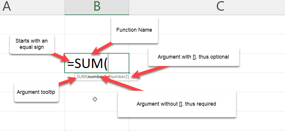
- Starts with the equals "=" sign
- Has a name. Some examples are VLOOKUP, SUM, UNIQUE, and XLOOKUP.
- Requires arguments which are separated by commas. You should know that semicolons are used as separators in countries like Spain, France, Italy, Netherlands, and Germany. You can, however, change this via the Excel setting.
- Argument with the square brackets [] are optional
- Has an opening and closing parenthesis.
- Has an argument tooltip which shows you what you should pass.
There are some exceptions. For example,
- The DATEDIF doesn't show in Excel because it is not a standard function and gives incorrect results in a few circumstances. However, here is the syntax:
DATEDIF(birthdate, TODAY(), "y")
- Functions like PI(), RAND(), NOW(), TODAY() require no argument.
How to Use Excel Functions
Let's look at a few functions:
How to Use the SUM() Function in Excel
According to the documentation, the SUM function adds values. Here is the syntax:
 Excel Sum Syntax
Let's assume that we have a line of numbers from 1 to 10 and we want to add it up. To achieve this, we will just type =SUM(A1:A10). The A1:A10 simply returns an array of number that are situated on cell A1 to A10 which are A1, A2, and A3 up through A10.

Since the second argument is optional, that means a sum(A10) will return a value. In our case, it will return just 10 since A10 has the value 10 in it. Give it a try.
If you were writing this using the addition operator, you would have written:
=1 + 2 + 3 + 4 + 5 + 6 + 7 + 8 + 9 + 10
or
=A1 + A2 + A3 + A4 + A5 + A6 + A7 + A8 + A9 + A10
This doesn't look very productive or efficient.
How to Use the TODAY() Function in Excel
According to the documentation, the TODAY function displays the current date on your worksheet. It also requires no argument. Here is the syntax:

Excel displays the current date automatically according to your computer's date and time setting. The same goes for the NOW() function, which displays the current date and time.
How to Use the CONCATENATE() Function in Excel
Let’s look at a text function. You use CONCATENATE to join two or more text strings into one string together.
Here is the syntax:
 Excel CONCATENATE() Syntax
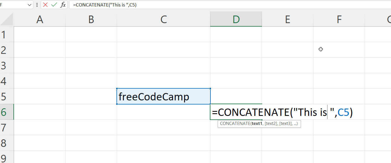
Let's assume we want to join “This is” with “freeCodeCamp” – but in your cell, you have just "freeCodeCamp."
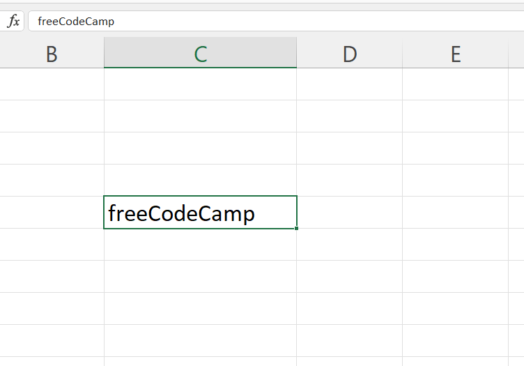 freeCodeCamp Excel
If you’re going to write a string inside a formula, you must write it inside quotes like this “ “.
Why?
This way, Excel wouldnt think you're trying to write another function.
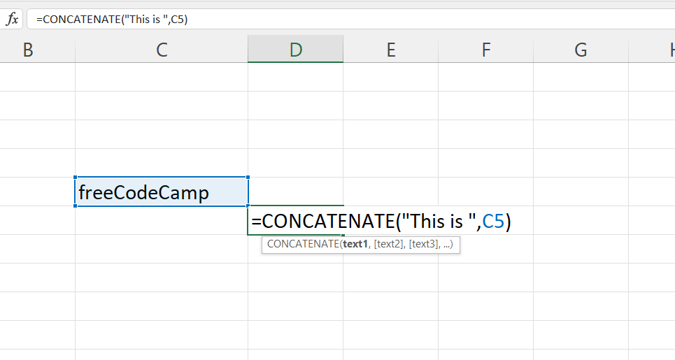 How to use Excel CONCATENATE function
This will return the phrase “This is freeCodeCamp”
 How to use CONCATENATE() in Excel
How to Use the VLOOKUP() Function in Excel
This is one of Excel’s most interesting and commonly used formulas or functions. You use it to find a value in a table or range by row.
Here is a scenario:
We have a simple table that shows various films along with their genre, lead studio, audience score %, profitability, rotten tomatoes %, worldwide gross and year. I would use just the first 10 rows of the sample data from this GitHub Gist.

I want that, whenever I type in a movie in the yellow cell, the year should get displayed in the green cell. Let's use VLOOKUP to find it.
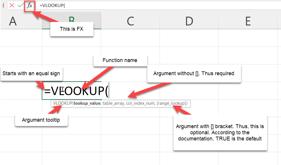
This is the VLOOKUP syntax:
 Excel Vlookup Syntax
Besides writing your formulas in the cell, you can also write them using the Excel Insert Function (fx) button, which is close to the formula bar.
Let's try this.
- Write
=Vlookup(on the green cell. - Click on fx. A dialogue box will pop up showing all the arguments this formula needs.
- Input the value for each argument.
- Lookup_value (required argument): This is what you want to find. In our case, that is the movie “Youth in Revolt” which is in cell B1.
- Table_array (required argument): This is just asking you for the table that contains the data. You give it the entire table, which in our case is A4:H13
- Col_index_num (required argument): This is asking you for the column number of the table you gave. In our case, we want the year. This is in column 8.
Range_lookup (optional argument): Lastly, we pick if we want an approximate match (TRUE) or an exact match (FALSE).
TRUE means approximate match, so it returns the closest or an estimate.
FALSE means exact match, so it returns an error if it's not found.
We would go for the FALSE because we want the exact match.

- Click on "OK." Excel will return 2010.
However, you can write this in the cell by typing in =VLOOKUP(B1,A4:H13,8,FALSE) in your cell.

Tips and Rules When Writing Excel Functions
When writing our function, Excel provides some formula tips.
- The Argument tooltip doesn't leave until you close the last parenthesis.
- The formula bar shows your formula.
- The argument you are currently writing is always dark. Take a look at the lookup_value in the image below.
- The square brackets [] tell you it is optional.
- Lastly, the colour code – our B1 is in blue, and cell B1 is in blue to guide us on what cell or table was picked. The same thing will happen to A4:H13 when we pick it as our table_array argument.

How to Work with Nested Functions in Excel
A nested function is when you write a function within another function. For example, finding the average of the sum of values.
The first tip when writing a nested function will be to treat every function individually. So address the first function before addressing the second. A pro tip would be to look at the argument tooltip when writing it.
Let's take a simple scenario.
We have two arrays of numbers. Each has the scores of students in the class. I want to add the two arrays before I get the average.
Let's get started.
- Type in your = followed by the average.
- The number one will be the sum of the scores from class one.
- The number two will be the sum of the scores from class two.
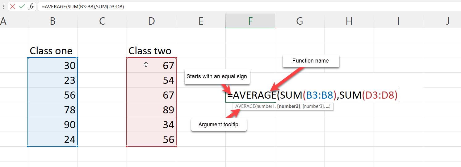 Nested Function: Excel AVERAGE and SUM syntax

Finally, don't forget the closing parenthesis.
Thus, the formula will be =AVERAGE(SUM(B3:B8),SUM(D3:D8)).
How to Work with Dynamic Array Functions in Excel
Dynamic array functions are formulas associated with spill array behaviour.
Before now, you wrote a function and it returned just a single input. We call these kinds of functions legacy array formulas.
Dynamic array functions, on the other hand, will return values that will enter the neighbouring cells. A few examples of dynamic array functions are:
- UNIQUE
- TEXTSPLIT
- FILTER
- SEQUENCE
- SORT
- SORTBY
- RANDARRAY
Let's look at the UNIQUE formula.
How to Use the UNIQUE() Formula in Excel
The unique formula works by returning the unique value from an array or list. Let's use the movie sample data from this GitHub Gist. This table contains 77 rows of film excluding the heading.

Let's try to get the unique years from our dataset – that is, years without duplicates.
To do this:
- Type
=UNIQUE( - Select the entire array of values from the year column: =UNIQUE(H2:H78)

- Close the parenthesis and press Enter.
Though the formula was written in a single cell, the returned value got spilled into the cells below it. That's the spilled array behaviour.

How to Create Your Own Functions in Excel
Microsoft Excel released a bunch of new functions to make user more productive. One of these function was the LAMBDA function.
The LAMBDA function lets you create custom functions without macros, VBA or JavaScript, and reuse them throughout a workbook.
The best part? you can name it.
How to Use the LAMBDA() Function in Excel
This LAMBDA function will increase productivity by eliminating the need to copy and paste this formula, which can be error-prone.
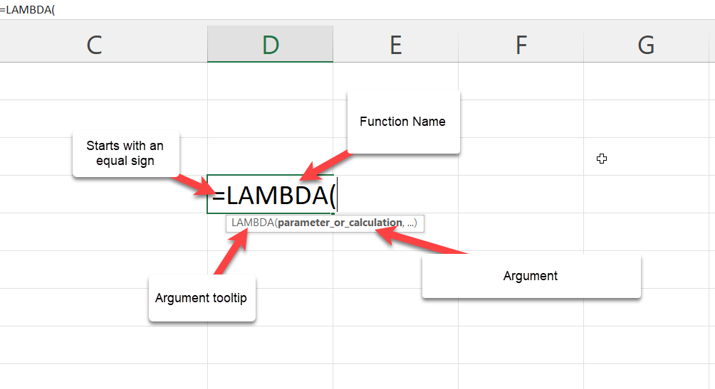
Here is the LAMBDA syntax:
 Excel LAMBDA function
Lets start with a simple use case using the movie sample data from this GitHub Gist.
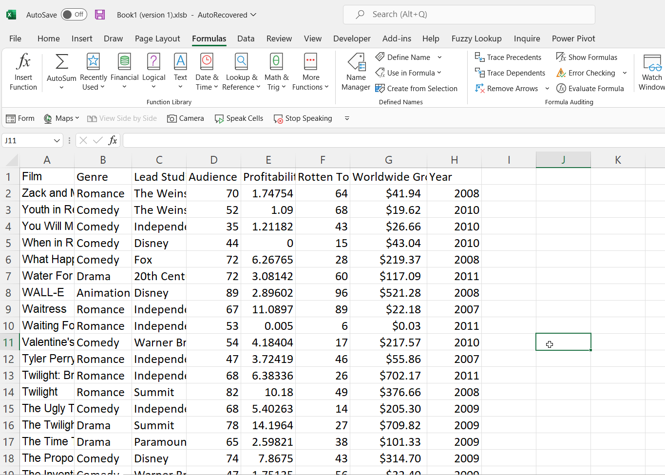 The Movie dataset
We had a column called "Worldwide Gross", lets try to find the Naira value.
- Create a new column and call it "Worldwide Gross in Naira".
- Right below our column name, Cell I2, type
=lAMBDA( - LAMBDA requires a parameter and/or a calculation.
The parameter means the value you want to pass, in our use case we want to change the gross value. Lets call it gross.
The calculation means the formula or function you want to execute. For us, that will be to multiply it with te exchange rate. At the moment, that's 670. so lets write gross * 670.
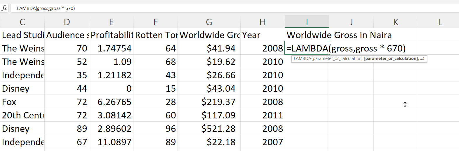 How to use LAMBDA function in Excel
- Press Enter. This will return an error because, gross doesnt exist and you need to let excel know of these names.
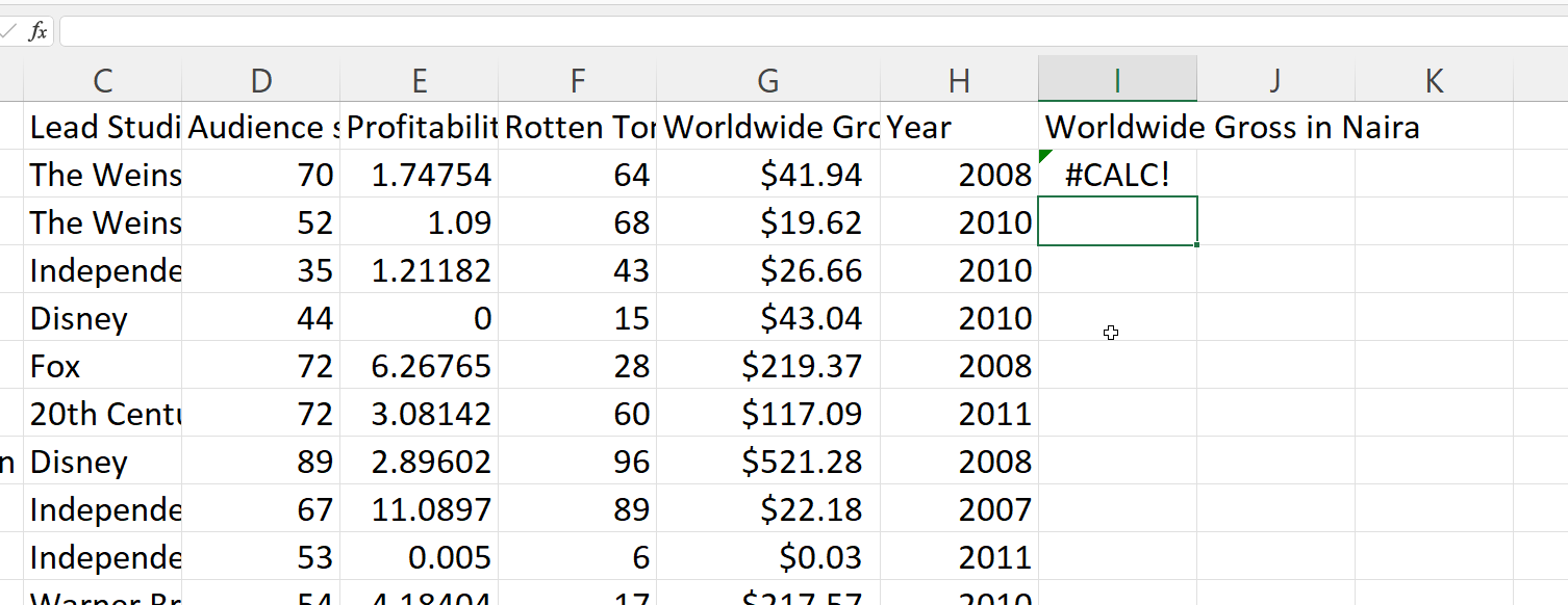 Using Excel LAMBDA
- To make use of the newly created function, you need to copy the syntax written.
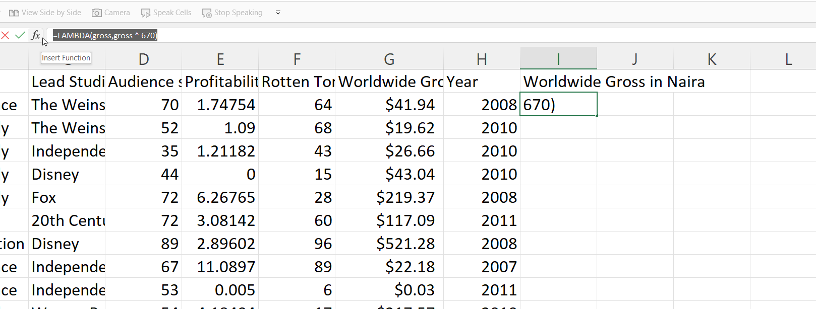 Writing function with Excel LAMBDA
- Go to the formula ribbon and open the name manager.
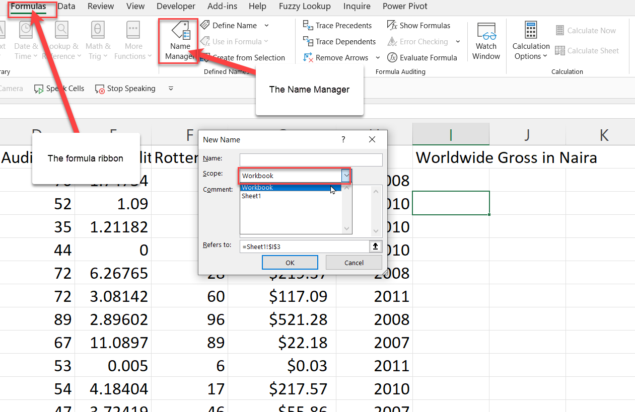 Excel name manger using the LAMBDA function
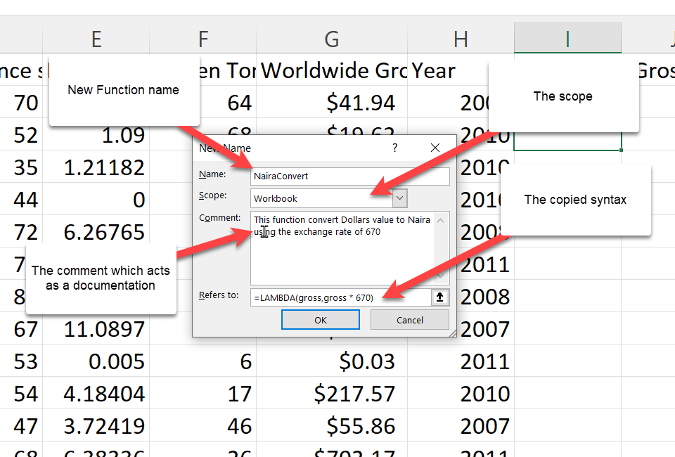
Define the name manger parameters:
The name is simply what you want to call this function. I am going with NairaConvert.
- The scope should be workbook because you want to use this function in the workbook.
- The comments explains what your function does. It is acts as a documentation.
- In the refer to, you should paste the copied function syntax.
 Excel name manager
Press Ok.
To use this new function, you call it with the name you defined it as—NairaConvert—and give it the gross which is our worldwise gross on G2.
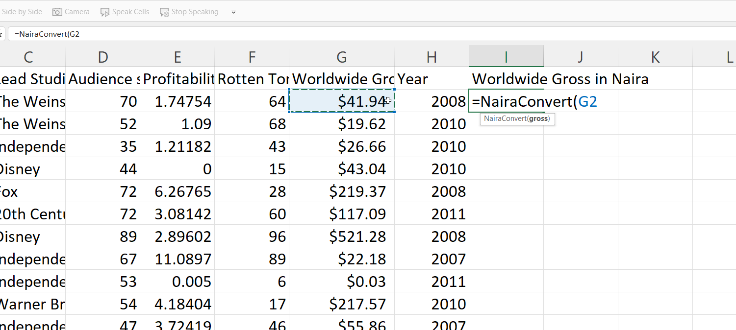 Custom function with LAMBDA
- Close the parenthesis and press Ok
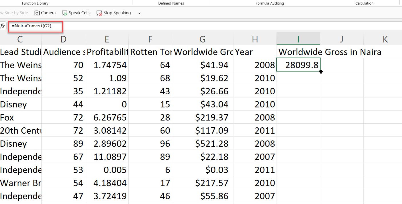 Calculating with Excel LAMBDA
Where Can I Learn More about Excel?
There are a ton of resources for learning Microsoft Excel nowadays. So many that it is hard to figure out which ones are up-to-date and helpful.
The best thing you can do is find a helpful tutorial and follow it to completion, instead of attempting to take several at once. I would advise you to start with freeCodeCamp's Microsoft Excel Tutorial for Beginners - Full Course, which is available on YouTube.
You should also join communities like the Microsoft Excel and Data Analysis Learning Community. However, if you’re looking for a compilation of resources, check out freeCodeCamp's publication Excel tags.
If you enjoyed reading this article and/or have any questions and want to connect, you can find me on LinkedIn or Twitter.