
By Andrey Germanov
Object detection is a computer vision task that involves identifying and locating objects in images or videos. It is an important part of many applications, such as self-driving cars, robotics, and video surveillance.
Over the years, many methods and algorithms have been developed to find objects in images and their positions. The best quality in performing these tasks comes from using convolutional neural networks.
One of the most popular neural networks for this task is YOLO, created in 2015 by Joseph Redmon, Santosh Divvala, Ross Girshick, and Ali Farhadi in their famous research paper "You Only Look Once: Unified, Real-Time Object Detection".
Since that time, there have been quite a few versions of YOLO. Recent releases can do even more than object detection. The newest release is YOLOv8, which we are going to use in this tutorial.
Here, I will show you the main features of this network for object detection. First, we will use a pre-trained model to detect common object classes like cats and dogs. Then, I will show how to train your own model to detect specific object types that you select, and how to prepare the data for this process. Finally, we will create a web application to detect objects on images right in a web browser using the custom trained model.
To follow this tutorial, you should be familiar with Python and have a basic understanding of machine learning, neural networks, and their application in object detection. You can watch this short video course to familiarize yourself with all required machine learning theory.
Once you've refreshed the theory, let's get started with the practice! Here's what we'll cover:
- Problems YOLOv8 Can Solve
- How to Get Started with YOLOv8
- How to Prepare Data to Train the YOLOv8 Model
- How to Train the YOLOv8 Model
- How to Create an Object Detection Web Service
- How to Create the Frontend
- How to Create the Backend
- Conclusion
Problems YOLOv8 Can Solve
You can use the YOLOv8 network to solve classification, object detection, and image segmentation problems. All these methods detect objects in images or in videos in different ways, as you can see in the image below:
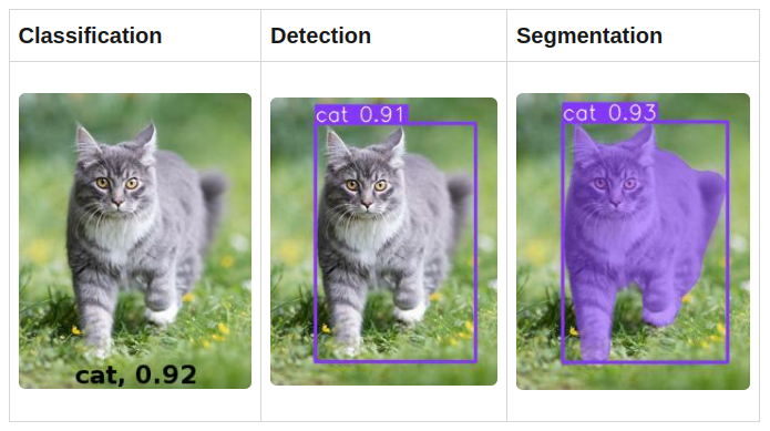 Common computer vision problems - classification, detection, and segmentation
The neural network that's created and trained for image classification determines a class of object on the image and returns its name and the probability of this prediction.
For example, on the left image, it returned that this is a "cat" and that the confidence level of this prediction is 92% (0.92).
The neural network for object detection, in addition to the object type and probability, returns the coordinates of the object on the image: x, y, width and height, as shown on the second image. Object detection neural networks can also detect several objects in the image and their bounding boxes.
Finally, in addition to object types and bounding boxes, the neural network trained for image segmentation detects the shapes of the objects, as shown on the right image.
There are many different neural network architectures developed for these tasks, and for each of them you had to use a separate network in the past. Fortunately, things changed after the YOLO created. Now you can use a single platform for all these problems.
In this article, we will explore object detection using YOLOv8. I will guide you through how to create a web application that will detect traffic lights and road signs in images. In later articles I will cover other features, including image segmentation.
In the next sections, we will go through all steps required to create an object detector. By the end of this tutorial, you will have a complete AI powered web application.
How to Get Started with YOLOv8
Technically speaking, YOLOv8 is a group of convolutional neural network models, created and trained using the PyTorch framework.
In addition, the YOLOv8 package provides a single Python API to work with all of them using the same methods. That is why, to use it, you need an environment to run Python code. I highly recommend using Jupyter Notebook.
After making sure that you have Python and Jupyter installed on your computer, run the notebook and install the YOLOv8 package in it by running the following command:
!pip install ultralytics
The ultralytics package has the YOLO class, used to create neural network models.
To get access to it, import it to your Python code:
from ultralytics import YOLO
Now everything is ready to create the neural network model:
model = YOLO("yolov8m.pt")
As I mentioned before, YOLOv8 is a group of neural network models. These models were created and trained using PyTorch and exported to files with the .pt extension.
There are three types of models and 5 models of different sizes for each type:
| Classification | Detection | Segmentation | Kind |
| yolov8n-cls.pt | yolov8n.pt | yolov8n-seg.pt | Nano |
| yolov8s-cls.pt | yolov8s.pt | yolov8s-seg.pt | Small |
| yolov8m-cls.pt | yolov8m.pt | yolov8m-seg.pt | Medium |
| yolov8l-cls.pt | yolov8l.pt | yolov8l-seg.pt | Large |
| yolov8x-cls.pt | yolov8x.pt | yolov8x-seg.pt | Huge |
The bigger the model you choose, the better the prediction quality you can achieve, but the slower it will work.
In this tutorial I will cover object detection – which is why, in the previous code snippet, I selected the "yolov8m.pt", which is a middle-sized model for object detection.
When you run this code for the first time, it will download the yolov8m.pt file from the Ultralytics server to the current folder. Then it will construct the model object. Now you can train this model, detect objects, and export it to use in production. For all these tasks, there are convenient methods:
- train({path to dataset descriptor file}) – used to train the model on the images dataset.
- predict({image}) – used to make a prediction for a specified image, for example to detect bounding boxes of all objects that the model can find in the image.
- export({format}) – used to export the model from the default PyTorch format to a specified format.
All YOLOv8 models for object detection ship already pre-trained on the COCO dataset, which is a huge collection of images of 80 different types. So, if you do not have specific needs, then you can just run it as is, without additional training.
For example, you can download this image as "cat_dog.jpg":
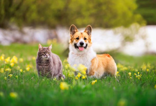 A sample image with cat and dog
and run predict to detect all objects in it:
results = model.predict("cat_dog.jpg")
The predict method accepts many different input types, including a path to a single image, an array of paths to images, the Image object of the well-known PIL Python library, and others.
After running the input through the model, it returns an array of results for each input image. As we provided only a single image, it returns an array with a single item that you can extract like this:
result = results[0]
The result contains detected objects and convenient properties to work with them. The most important one is the boxes array with information about detected bounding boxes on the image. You can determine how many objects it detected by running the len function:
len(result.boxes)
When I ran this, I got "2", which means that there are two boxes detected: one for the dog and one for the cat.
Then you can analyze each box either in a loop or manually. Let's get the first one:
box = result.boxes[0]
The box object contains the properties of the bounding box, including:
xyxy– the coordinates of the box as an array [x1,y1,x2,y2]cls– the ID of object typeconf– the confidence level of the model about this object. If it's very low, like < 0.5, then you can just ignore the box.
Let's print information about the detected box:
print("Object type:", box.cls)
print("Coordinates:", box.xyxy)
print("Probability:", box.conf)
For the first box, you will receive the following information:
Object type: tensor([16.])
Coordinates: tensor([[261.1901,  94.3429, 460.5649, 312.9910]])
Probability: tensor([0.9528])
As I explained above, YOLOv8 contains PyTorch models. The outputs from the PyTorch models are encoded as an array of PyTorch Tensor objects, so you need to extract the first item from each of these arrays:
print("Object type:",box.cls[0])
print("Coordinates:",box.xyxy[0])
print("Probability:",box.conf[0])
Object type: tensor(16.)
Coordinates: tensor([261.1901,  94.3429, 460.5649, 312.9910])
Probability: tensor(0.9528)
Now you see the data as Tensor objects. To unpack actual values from Tensor, you need to use the .tolist() method for tensors with array inside, as well as the .item() method for tensors with scalar values.
Let's extract the data to the appropriate variables:
cords = box.xyxy[0].tolist()
class_id = box.cls[0].item()
conf = box.conf[0].item()
print("Object type:", class_id)
print("Coordinates:", cords)
print("Probability:", conf)
Object type: 16.0
Coordinates: [261.1900634765625, 94.3428955078125, 460.5649108886719, 312.9909973144531]
Probability: 0.9528293609619141
Now you see the actual data. The coordinates can be rounded, and the probability also can be rounded to two digits after the dot.
The object type is 16 here. What does this mean? Let's talk more about that.
All objects that the neural network can detect have numeric IDs. In case of a YOLOv8 pretrained model, there are 80 object types with IDs from 0 to 79. The COCO object classes are well known and you can easily google them on the Internet. In addition, the YOLOv8 result object contains the convenient names property to get these classes:
print(result.names)
{0: 'person',
 1: 'bicycle',
 2: 'car',
 3: 'motorcycle',
 4: 'airplane',
 5: 'bus',
 6: 'train',
 7: 'truck',
 8: 'boat',
 9: 'traffic light',
 10: 'fire hydrant',
 11: 'stop sign',
 12: 'parking meter',
 13: 'bench',
 14: 'bird',
 15: 'cat',
 16: 'dog',
 17: 'horse',
 18: 'sheep',
 19: 'cow',
 20: 'elephant',
 21: 'bear',
 22: 'zebra',
 23: 'giraffe',
 24: 'backpack',
 25: 'umbrella',
 26: 'handbag',
 27: 'tie',
 28: 'suitcase',
 29: 'frisbee',
 30: 'skis',
 31: 'snowboard',
 32: 'sports ball',
 33: 'kite',
 34: 'baseball bat',
 35: 'baseball glove',
 36: 'skateboard',
 37: 'surfboard',
 38: 'tennis racket',
 39: 'bottle',
 40: 'wine glass',
 41: 'cup',
 42: 'fork',
 43: 'knife',
 44: 'spoon',
 45: 'bowl',
 46: 'banana',
 47: 'apple',
 48: 'sandwich',
 49: 'orange',
 50: 'broccoli',
 51: 'carrot',
 52: 'hot dog',
 53: 'pizza',
 54: 'donut',
 55: 'cake',
 56: 'chair',
 57: 'couch',
 58: 'potted plant',
 59: 'bed',
 60: 'dining table',
 61: 'toilet',
 62: 'tv',
 63: 'laptop',
 64: 'mouse',
 65: 'remote',
 66: 'keyboard',
 67: 'cell phone',
 68: 'microwave',
 69: 'oven',
 70: 'toaster',
 71: 'sink',
 72: 'refrigerator',
 73: 'book',
 74: 'clock',
 75: 'vase',
 76: 'scissors',
 77: 'teddy bear',
 78: 'hair drier',
 79: 'toothbrush'}
This dictionary has everything that this model can detect. Now you can find that 16 is "dog", so this bounding box is the bounding box for detected DOG.
Let's modify the output to show results in a more representative way:
cords = box.xyxy[0].tolist()
cords = [round(x) for x in cords]
class_id = result.names[box.cls[0].item()]
conf = round(box.conf[0].item(), 2)
print("Object type:", class_id)
print("Coordinates:", cords)
print("Probability:", conf)
In this code I rounded all coordinates using Python list comprehension. Then I got the name of the detected object class by ID using the result.names dictionary. I also rounded the probability. You should get the following output:
Object type: dog
Coordinates: [261, 94, 461, 313]
Probability: 0.95
This data is good enough to show in the user interface. Let's now write some code to get this information for all detected boxes in a loop:
for box in result.boxes:
  class_id = result.names[box.cls[0].item()]
  cords = box.xyxy[0].tolist()
  cords = [round(x) for x in cords]
  conf = round(box.conf[0].item(), 2)
  print("Object type:", class_id)
  print("Coordinates:", cords)
  print("Probability:", conf)
  print("---")
This code will do the same for each box and will output the following:
Object type: dog
Coordinates: [261, 94, 461, 313]
Probability: 0.95
---
Object type: cat
Coordinates: [140, 170, 256, 316]
Probability: 0.92
---
This way you can run object detection for other images and see everything that a COCO-trained model can detect in them.
This video shows the whole coding session of this section in Jupyter Notebook, assuming you have it installed.
Using models that are pre-trained on well-known objects is ok to start. But in practice, you may need a solution to detect specific objects for a concrete business problem.
For example, someone may need to detect specific products on supermarket shelves or discover brain tumors on x-rays. It's highly likely that this information is not available in public datasets, and there are no free models that know about everything.
So, you have to teach your own model to detect these types of objects. To do that, you need to create a database of annotated images for your problem and train the model on these images.
How to Prepare Data to Train the YOLOv8 Model
To train the model, you need to prepare annotated images and split them into training and validation datasets.
You'll use the training set to teach the model and the validation set to test the results of the study and measure the quality of the trained model. You can put 80% of the images in the training set and 20% in the validation set.
These are the steps that you need to follow to create each of the datasets:
- Decide on and encode classes of objects you want to teach your model to detect. For example, if you want to detect only cats and dogs, then you can state that "0" is cat and "1" is dog.
- Create a folder for your dataset and two subfolders in it: "images" and "labels".
- Add the images to the "images" subfolder. The more images you collect, the better for training.
- For each image, create an annotation text file in the "labels" subfolder. Annotation text files should have the same names as image files and the ".txt" extensions. In the annotation files you should add records about each object that exist on the appropriate image in the following format:
{object_class_id} {x_center} {y_center} {width} {height}
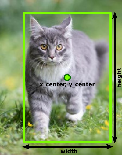 Bounding box parameters
This is the most time-consuming manual work in the machine learning process: to measure bounding boxes for all objects and add them to annotation files.
You should also normalize the coordinates to fit in a range from 0 to 1. To calculate them, you need to use the following formulas:
- x_center = (box_x_left+box_x_width/2)/image_width
- y_center = (box_y_top+box_height/2)/image_height
- width = box_width/image_width
- height = box_height/image_height
For example, if you want to add the "cat_dog.jpg" image that we used before to the dataset, you need to copy it to the "images" folder and then measure and collect the following data about the image, and it's bounding boxes:
Image:
image_width = 612
image_height = 415
Objects:
| Dog | Cat |
|
box_x_left=261 box_x_top=94 box_width=200 box_height=219 |
box_x_left=140 box_x_top=170 box_width=116 box_height=146 |
Then, create the "cat_dog.txt" file in the "labels" folder and, using the formulas above, calculate the coordinates:
Dog (class id=1):
x_center = (261+200/2)/612 = 0.589869281
y_center = (94+219/2)/415 = 0.490361446
width = 200/612 = 0.326797386
height = 219/415 = 0.527710843
Cat (class id=0)
x_center = (140+116/2)/612 = 0.323529412
y_center = (170+146/2)/415 = 0.585542169
width = 116/612 = 0.189542484
height = 146/415 = 0.351807229
and add the following lines to the file:
1 0.589869281 0.490361446 0.326797386 0.527710843
0 0.323529412 0.585542169 0.189542484 0.351807229
The first line contains a bounding box for the dog (class id=1). The second line contains a bounding box for the cat (class id=0). Of course, you can have the image with many dogs and many cats at the same time, and you can add bounding boxes for all of them.
After adding and annotating all images, the dataset is ready. You need to create two datasets and place them in different folders. The final folder structure can look like this:
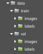 Dataset structure
As you can see, the training dataset is located in the "train" folder and the validation dataset is located in the "val" folder.
Finally, you need to create a dataset descriptor YAML-file that points to the created datasets and describes the object classes in them. This is a sample of this file for the data created above:
train: ../train/images
val: ../val/images

nc: 2
names: ['cat','dog']
In the first two lines, you need to specify paths to the images of the training and the validation datasets. The paths can be either relative to the current folder or absolute.
Then, the nc line specifies the number of classes that exist in these datasets, and names is an array of class names in correct order.
Indexes of these items are numbers that you used when annotating the images, and these indexes will be returned by the model when it detects objects using the predict method. So, if you used "0" for cats, then it should be the first item in the names array.
This YAML file should be passed to the train method of the model to start the training process.
To make the image annotation process easier, there are a lot of programs you can use to visually annotate images for machine learning. You can search for something like "software to annotate images for machine learning" to get a list of these programs.
There are also many online tools that can do all this work, like Roboflow Annotate. Using this service, you just need to upload your images, draw bounding boxes on them, and set classes for each bounding box. Then, the tool will automatically create annotation files, split your data to train and validation datasets, and create a YAML descriptor file. Then you can export and download the annotated data as a ZIP file.
In the below video, I show you how to use Roboflow to create the "cats and dogs" micro-dataset.
For real life problems, that database should be much bigger. To train a good model, you should have hundreds or thousands of annotated images.
Also, when preparing the images database, try to make it balanced. It should have an equal number of objects of each class, that is an equal number of dogs and cats in this example. Otherwise, the model trained on it may predict one class better than another.
After the data is ready, copy it to the folder with your Python code that you will use for training and return back to your Jupyter Notebook to start the training process.
How to Train the YOLOv8 Model
After the data is ready, you need to pass it through the model. To make it more interesting, we will not use this small "cats and dogs" dataset. We will use another custom dataset for training that contains traffic lights and road signs. This is a free dataset that I got from the Roboflow Universe. Press "Download Dataset" and select "YOLOv8" as the format.
If it's not available on Roboflow when you read this, then you can get it from my Google Drive. You can use this dataset to teach YOLOv8 to detect different objects on roads, like you can see in the next screenshot.
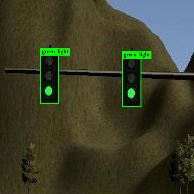 Traffic lights detection demo
You can open the downloaded zip file and ensure that it's already annotated and structured using the rules described above. You can find the dataset descriptor file data.yaml in the archive as well.
If you downloaded the archive from Roboflow, it will contain the additional "test" dataset, which is not used by the training process. You can use the images from it for additional testing on your own after training.
Extract the archive to the folder with your Python code and execute the train method to start a training loop:
model.train(data="data.yaml", epochs=30)
The data is the only required option. You have to pass the YAML descriptor file to it. The epochs option specifies the number of training cycles (100 by default). There are other options that can affect the process and quality of the trained model.
Each training cycle consists of two phases: a training phase and a validation phase.
During the training phase, the train method does the following:
- Extracts the random batch of images from the training dataset (the number of images in the batch can be specified using the
batchoption). - Passes these images through the model and receives the resulting bounding boxes of all detected objects and their classes.
- Passes the result to the loss function that's used to compare the received output with correct result from annotation files for these images. The loss function calculates the amount of error.
- The result of the loss function is passed to the
optimizerto adjust the model weights based on the amount of error in the correct direction. This reduces the errors in the next cycle. By default, the SGD (Stochastic Gradient Descent) optimizer is used, but you can try others, like Adam, to see the difference.
During the validation phase, train does the following:
- Extracts the images from the validation dataset.
- Passes them through the model and receives the detected bounding boxes for these images.
- Compares the received result with true values for these images from annotation text files.
- Calculates the precision of the model based on the difference between actual and expected results.
The progress and results of each phase for each epoch are displayed on the screen. This way you can see how the model learns and improves from epoch to epoch.
When you run the train code, you will see a similar output to the following during the training loop:
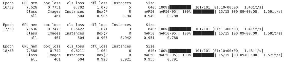 Training process
For each epoch it shows a summary for both the training and validation phases: lines 1 and 2 show results of the training phase and lines 3 and 4 show the results of the validation phase for each epoch.
The training phase includes a calculation of the amount of error in a loss function, so the most valuable metrics here are box_loss and cls_loss.
box_lossshows the amount of error in detected bounding boxes.cls_lossshows the amount of error in detected object classes.
Why is the loss split to different metrics? Because the model might correctly detect the bounding box coordinates around the object, but incorrectly detect the object class in this box. For example, in my practice, it detected the dog as a horse, but the dimensions of the object were detected correctly.
If the model really learns something from the data, then you should see that these values decrease from epoch to epoch. In a previous screenshot the box_loss decreased: 0.7751, 0.7473, 0.742 and the cls_loss decreased too: 0.702, 0.6422, 0.6211.
In the validation phase, it calculates the quality of the model after training using the images from the validation dataset.
The most valuable quality metric is mAP50-95, which is Mean Average Precision. If the model learns and improves, the precision should grow from epoch to epoch. In a previous screenshot you can see that it slowly grew: 0.788, 0.788, 0.791.
If after the last epoch you did not get acceptable precision, you can increase the number of epochs and run the training again. Also, you can tune other parameters like batch, lr0, lrf or change the optimizer you're using. There are no clear rules on what to do here, but there are a lot of recommendations.
The topic of tuning the parameters of the training process goes beyond the scope of article. I think it's possible to write a book about this and many of them already exist. You can easily find them on the Internet. But in a few words, most of them say that you need to experiment and try all possible options and compare results.
In addition to the metrics that are shown during the training process, it writes a lot of statistics on disk. When training starts, it creates the runs/detect/train subfolder in the current folder and after each epoch it logs different log files to it.
It also exports the trained model after each epoch to the /runs/detect/train/weights/last.pt file and the model with the highest precision to the /runs/detect/train/weights/best.pt file. So, after training is finished, you can get the best.pt file to use in production.
You can watch this video to learn more about how the training process works. I used Google Colab which is a cloud version of Jupyter Notebook to get access to hardware with more powerful GPU to speed up the training process.
The video shows how to train the model on 5 epochs and download the final best.pt model. In real world problems, you need to run much more epochs and be prepared to wait hours or maybe days until training finishes.
After it's finished, it's time to run the trained model in production. In the next section, we will create a web service to detect objects in images online in a web browser.
How to Create an Object Detection Web Service
At this point, we're finished experimenting with the model in the Jupyter Notebook. You'll need to write the next batch of code as a separate project, using any Python IDE like VS Code or PyCharm.
The web service that we are going to create will have a web page with a file input field and an HTML5 canvas element.
When the user selects an image file using the input field, the interface will send it to the backend. Then, the backend will pass the image through the model that we created and trained and return the array of detected bounding boxes to the web page.
When it receives this, the frontend will draw the image on the canvas element and the detected bounding boxes on top of it.
The service will look and work as demonstrated on this video:
In the video, I used the model trained on 30 epochs, and it still does not detect some traffic lights. You can try to train it more to get better results. But the best way to improve the quality of a machine learning model is by adding more and more data.
So, as an additional exercise, you can import the dataset folder to Roboflow, add and annotate more images to it, and then use the updated data to continue training the model.
How to Create the Frontend
To start with, create a folder for a new Python project and an index.html file in it for the frontend web page. Here are the contents of this file:
<!DOCTYPE html>
<html lang="en">
<head>
    <meta charset="UTF-8">
    <title>YOLOv8 Object Detection</title>
    <style>
        canvas {
            display:block;
            border: 1px solid black;
            margin-top:10px;
        }
    </style>
</head>
<body>
    <input id="uploadInput" type="file"/>
    <canvas></canvas>
    <script>
       /**
       * "Upload" button onClick handler: uploads selected
       * image file to backend, receives an array of
       * detected objects and draws them on top of image
       */
       const input = document.getElementById("uploadInput");
       input.addEventListener("change",async(event) => {
           const file = event.target.files[0];
           const data = new FormData();
           data.append("image_file",file,"image_file");
           const response = await fetch("/detect",{
               method:"post",
               body:data
           });
           const boxes = await response.json();
           draw_image_and_boxes(file,boxes);
       })

       /**
       * Function draws the image from provided file
       * and bounding boxes of detected objects on
       * top of the image
       * @param file Uploaded file object
       * @param boxes Array of bounding boxes in format
         [[x1,y1,x2,y2,object_type,probability],...]
       */
       function draw_image_and_boxes(file,boxes) {
          const img = new Image()
          img.src = URL.createObjectURL(file);
          img.onload = () => {
              const canvas = document.querySelector("canvas");
              canvas.width = img.width;
              canvas.height = img.height;
              const ctx = canvas.getContext("2d");
              ctx.drawImage(img,0,0);
              ctx.strokeStyle = "#00FF00";
              ctx.lineWidth = 3;
              ctx.font = "18px serif";
              boxes.forEach(([x1,y1,x2,y2,label]) => {
                  ctx.strokeRect(x1,y1,x2-x1,y2-y1);
                  ctx.fillStyle = "#00ff00";
                  const width = ctx.measureText(label).width;
                  ctx.fillRect(x1,y1,width+10,25);
                  ctx.fillStyle = "#000000";
                  ctx.fillText(label,x1,y1+18);
              });
          }
       }
  </script>
</body>
</html>
The HTML part is very tiny and consists only of the file input field with "uploadInput" ID and the canvas element below it.
Then, in the JavaScript part, the "onChange" we define the event handler for the input field. When the user selects an image file, the handler uses fetch to make a POST request to the /detect backend endpoint (which we will create later) and sends this image file to it.
The backend should detect objects on this image and return a response with a boxes array as JSON. This response then gets decoded and passed to the draw_image_and_boxes function along with an image file itself.
The draw_image_and_boxes function loads the image from file. As soon as it's loaded, it draws it on the canvas. Then, it draws each bounding box with a class label on top of the canvas with the image.
So, now let's create the backend with a /detect endpoint for it.
How to Create the Backend
We'll create the backend using Flask. Flask has its own internal web server, but according to many Flask developers, it's not reliable enough for productio. So we will use the Waitress web server and run our Flask app in it.
Also, we will use the Pillow library to read an uploaded binary files as images. Make sure you have all these packages installed on your system before continuing:
pip3 install flask
pip3 install waitress
pip3 install pillow
The backend will be in a single file. Let's name it object_detector.py:
from ultralytics import YOLO
from flask import request, Response, Flask
from waitress import serve
from PIL import Image
import json

app = Flask(__name__)

@app.route("/")
def root():
    """
    Site main page handler function.
    :return: Content of index.html file
    """
    with open("index.html") as file:
        return file.read()


@app.route("/detect", methods=["POST"])
def detect():
    """
        Handler of /detect POST endpoint
        Receives uploaded file with a name "image_file",
        passes it through YOLOv8 object detection
        network and returns an array of bounding boxes.
        :return: a JSON array of objects bounding
        boxes in format
        [[x1,y1,x2,y2,object_type,probability],..]
    """
    buf = request.files["image_file"]
    boxes = detect_objects_on_image(Image.open(buf.stream))
    return Response(
      json.dumps(boxes),
      mimetype='application/json'
    )


def detect_objects_on_image(buf):
    """
    Function receives an image,
    passes it through YOLOv8 neural network
    and returns an array of detected objects
    and their bounding boxes
    :param buf: Input image file stream
    :return: Array of bounding boxes in format
    [[x1,y1,x2,y2,object_type,probability],..]
    """
    model = YOLO("best.pt")
    results = model.predict(buf)
    result = results[0]
    output = []
    for box in result.boxes:
        x1, y1, x2, y2 = [
          round(x) for x in box.xyxy[0].tolist()
        ]
        class_id = box.cls[0].item()
        prob = round(box.conf[0].item(), 2)
        output.append([
          x1, y1, x2, y2, result.names[class_id], prob
        ])
    return output

serve(app, host='0.0.0.0', port=8080)
First, we import the required libraries:
- ultralytics for the YOLOv8 model.
- flask to create a
Flaskweb application, to receiverequestsfrom the frontend and sendresponsesback to it. - waitress to run a web server and
servethe Flask webappin it. - PIL to load an uploaded file as an
Imageobject, that required for YOLOv8. - json to convert the array of bounding boxes to JSON before returning it to the frontend.
Then, we defined two routes:
/that serves as a root of web service. It just returns the content of the "index.html" file./detectthat responds to an image upload request from the frontend. It converts the RAW file to the Pillow Image object, then passes this image to thedetect_objects_on_imagefunction.
The detect_objects_on_image function creates a model object based on the best.pt model that we trained in the previous section. Make sure that this file exists in the folder where you write the code.
Then it calls the predict method for the image. predict returns the detected bounding boxes.
Next, for each box it extracts the coordinates, class name, and probability in the same way as we did in the beginning of the tutorial. It adds this info to the output array.
Finally, the function returns the array of detected object coordinates and their classes.
After this, the array gets encoded to JSON and is returned to the frontend.
The last line of code starts the web server on port 8080 that serves the app Flask application.
To run the service, execute the following command:
python3 object_detector.py
If everything is working properly, you can open http:///localhost:8080 in a web browser. It should show the index.html page. When you select any image file, it will process it and display bounding boxes around all detected objects (or just display the image if nothing is detected on it).
The web service we just created is universal. You can use it with any YOLOv8 model. At the moment, it detects traffic lights and road signs using the best.pt model we created. But you can change it to use another model, like the yolov8m.pt model we used earlier to detect cats, dogs, and all other object classes that pretrained YOLOv8 models can detect.
Conclusion
In this tutorial, I guided you thought a process of creating an AI powered web application that uses the YOLOv8, a state-of-the-art convolutional neural network for object detection.
I showed you how to create models using the pre-trained models and prepare the data to train custom models. And finally we created a web application with a frontend and backend that uses the custom trained YOLOv8 model to detect traffic lights and road signs.
You can find a source code of this app in this GitHub repository.
For all these tasks, we used the Ultralytics high level APIs that come with the YOLOv8 package by default. These APIs are based on the PyTorch framework, which was used to create the bigger part of today's neural networks.
It's quite convenient on the one hand, but dependence on these high level APIs has a negative effect as well. If you need to run this web app in production, you should install all these environments there, including Python, PyTorch and the other dependencies.
To run this on a clean new server, you'll need to download and install more than 1 GB of third party libraries! This is definitely not the best way to go.
Also, what if you do not have Python in your production environment? What if all your other code is written in another programming language, and you do not plan to use Python? Or what if you want to run the model on a mobile phone with Android or iOS?
All this is to say that using Ultralytics packages is great for experimenting, training, and preparing the models for production. But in production itself, you have to load and use the model directly and not use those high-level APIs.
To do this, you need to understand how the YOLOv8 neural network works under the hood and write more code to provide input to the model and to process the output from it. This will make your apps faster and less resource-intense. You will not need to have PyTorch installed to run your object detection model.
Also, you will be able to run your models even without Python, using many other programming languages, including Julia, C++, Go, Node.js on backend, or even without backend at all. You can run the YOLOv8 models right in a browser, using only JavaScript on frontend.
Want to know how? This will be the topic of my next article about YOLOv8.
You can find me on LinkedIn, Twitter, and Facebook to know first about new articles like this one and other software development news.
Have a fun coding and never stop learning!