How to Detect Outliers in Machine Learning – 4 Methods for Outlier Detection

Have you ever trained a machine learning model on a real-world dataset? If yes, you’ll have likely come across outliers.

Outliers are those data points that are significantly different from the rest of the dataset. They are often abnormal observations that skew the data distribution, and arise due to inconsistent data entry, or erroneous observations.

To ensure that the trained model generalizes well to the valid range of test inputs, it’s important to detect and remove outliers.

In this guide, we’ll explore some statistical techniques that are widely used for outlier detection and removal.

Why Should You Detect Outliers?

In the machine learning pipeline, data cleaning and preprocessing is an important step as it helps you better understand the data. During this step, you deal with missing values, detect outliers, and more.

As outliers are very different values—abnormally low or abnormally high—their presence can often skew the results of statistical analyses on the dataset. This could lead to less effective and less useful models.

But dealing with outliers often requires domain expertise, and none of the outlier detection techniques should be applied without understanding the data distribution and the use case.

For example, in a dataset of house prices, if you find a few houses priced at around $1.5 million—much higher than the median house price, they’re likely outliers. However, if the dataset contains a significantly large number of houses priced at $1 million and above—they may be indicative of an increasing trend in house prices. So it would be incorrect to label them all as outliers. In this case, you need some knowledge of the real estate domain.

The goal of outlier detection is to remove the points—which are truly outliers—so you can build a model that performs well on unseen test data. We’ll go over a few techniques that’ll help us detect outliers in data.

How to Detect Outliers Using Standard Deviation

When the data, or certain features in the dataset, follow a normal distribution, you can use the standard deviation of the data, or the equivalent z-score to detect outliers.

In statistics, standard deviation measures the spread of data around the mean, and in essence, it captures how far away from the mean the data points are.

For data that is normally distributed, around 68.2% of the data will lie within one standard deviation from the mean. Close to 95.4% and 99.7% of the data lie within two and three standard deviations from the mean, respectively.

Let’s denote the standard deviation of the distribution by σ, and the mean by μ.

One approach to outlier detection is to set the lower limit to three standard deviations below the mean (μ - 3*σ), and the upper limit to three standard deviations above the mean (μ + 3*σ). Any data point that falls outside this range is detected as an outlier.

As 99.7% of the data typically lies within three standard deviations, the number of outliers will be close to 0.3% of the size of the dataset.

Code for Outlier Detection Using Standard Deviation

Now, let's create a normally-distributed dataset of student scores, and perform outlier detection on it.

As a first step, we’ll import the necessary modules.

import numpy as np
import pandas as pd
import seaborn as sns

Next, let’s define the function generate_scores() that returns a normally-distributed dataset of student scores containing 200 records. We’ll make a call to the function, and store the returned array in the variable scores_data.

def generate_scores(mean=60,std_dev=12,num_samples=200):
	np.random.seed(27)
	scores = np.random.normal(loc=mean,scale=std_dev,size=num_samples)
	scores = np.round(scores, decimals=0)
	return scores
scores_data = generate_scores()

You can use Seaborn’s displot() function to visualize the data distribution. In this case, the dataset follows a normal distribution, as seen in the figure below.

sns.set_theme()
sns.displot(data=scores_data).set(title="Distribution of Scores", xlabel="Scores")

Next, let's load the data into a Pandas dataframe for further analysis.

df_scores = pd.DataFrame(scores_data,columns=['score'])

To obtain the mean and standard deviation of the data in the dataframe df_scores, you can use the .mean() and the .std() methods, respectively.

df_scores.mean()
# Output
score    61.005
dtype: float64
df_scores.std()
# Output
score    11.854434
dtype: float64

As discussed earlier, set the lower limit (lower_limit) to be three standard deviations below the mean, and the upper limit (upper_limit) to be three standard deviations above the mean.

lower_limit = df_scores.mean() - 3*df_scores.std()
upper_limit = df_scores.mean() + 3*df_scores.std()
print(lower_limit)
print(upper_limit)
# Output
25.530716709142666
96.47928329085734

Now that you’ve defined the lower and upper limits, you may filter the dataframe df_scores to only retain the data points in the interval [lower_limit, upper_limit], as shown below.

df_scores_filtered=df_scores[(df_scores['score']>lower_limit)&(df_scores['score']<upper_limit)]
print(df_scores_filtered)
# Output
score
0     75.0
1     56.0
2     67.0
3     65.0
4     63.0
..     ...
194   42.0
195   76.0
196   67.0
197   74.0
199   53.0
[198 rows x 1 columns]

From the output above, you can see that two records have been removed, and df_scores_filtered contains 198 records.

How to Detect Outliers Using the Z-Score

Now let's explore the concept of the z-score. For a normal distribution with mean μ and standard deviation σ, the z-score for a value x in the dataset is given by:

z = (x - μ)/σ

From the above equation, we have the following:

• When x = μ, the value of z-score is 0.
• When x = μ ± 1, μ ± 2, or μ ± 3, the z-score is ± 1, ± 2, or ± 3, respectively.

Notice how this technique is equivalent to the scores based on standard deviation we had earlier. Under this transformation, all data points that lie below the lower limit, μ - 3*σ, now map to points that are less than -3 on the z-score scale.

Similarly, all points that lie above the upper limit, μ + 3*σ map to a value above 3 on the z-score scale. So [lower_limit, upper_limit] becomes [-3, 3].

Let’s use this technique on our dataset of scores.

Code for Outlier Detection Using Z-Score

Let's compute z-scores for all points in the dataset, and add z_score as a column to the dataframe df_scores.

df_scores['z_score']=(df_scores['score'] - df_scores['score'].mean())/df_scores['score'].std()
df_scores.head()
# Output
score	z_score
0	75.0	1.180571
1	56.0	-0.422205
2	67.0	0.505718
3	65.0	0.337005
4	63.0	0.168291

You can filter the dataframe df_scores to retain points whose z-scores are in the range [-3, 3], as shown below. The filtered dataframe contains 198 records, as expected.

df_scores_filtered= df_scores[(df_scores['z_score']>-3) & (df_scores['z_score']<3)]

print(df_scores_filtered)

# Output
     score   z_score

0     75.0  1.180571

1     56.0 -0.422205

2     67.0  0.505718

3     65.0  0.337005

4     63.0  0.168291

..     ...       ...

194   42.0 -1.603198

195   76.0  1.264928

196   67.0  0.505718

197   74.0  1.096214

199   53.0 -0.675275


[198 rows x 2 columns]

The methods involving standard deviation and z-scores can be used only when the data set, or the feature that you are examining, follows a normal distribution.

Next, we’ll discuss two outlier detection techniques that can be used independently of the data distribution.

How to Detect Outliers Using the Interquartile Range (IQR)

In statistics, interquartile range or IQR is a quantity that measures the difference between the first and the third quartiles in a given dataset.

• The first quartile is also called the one-fourth quartile, or the 25% quartile.
• If q25 is the first quartile, it means 25% of the points in the dataset have values less than q25.
• The third quartile is also called the three-fourth, or the 75% quartile.
• If q75 is the three-fourth quartile, 75% of the points have values less than q75.
• Using the above notations, IQR = q75 - q25.

Code for Outlier Detection Using Interquartile Range (IQR)

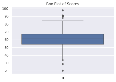
You can use the box plot, or the box and whisker plot, to explore the dataset and visualize the presence of outliers. The points that lie beyond the whiskers are detected as outliers.

You can generate box plots in Seaborn using the boxplot function.

sns.boxplot(data=scores_data).set(title="Box Plot of Scores")

Now, call the describe method on the dataframe df_scores.

df_scores.describe()
# Output
score
count	200.000000
mean	61.005000
std	    11.854434
min	    20.000000
25%	    54.000000
50%	    62.000000
75%	    67.000000
max	    98.000000

We use the 25% and 75% quartile values from the above result to compute IQR, and subsequently set the lower and upper limits to filter df_scores.

IQR = 67-54
lower_limit = 54 - 1.5*IQR
upper_limit = 67 + 1.5*IQR
print(upper_limit)
print(lower_limit)
# Output
86.5
34.5

As a next step, filter the dataframe df_scores to retain records that lie in the permissible range.

df_scores_filtered = df_scores[(df_scores['score']>lower_limit) & (df_scores['score']<upper_limit)]
print(df_scores_filtered)
# Output
score
0     75.0
1     56.0
2     67.0
3     65.0
4     63.0
..     ...
194   42.0
195   76.0
196   67.0
197   74.0
199   53.0
[192 rows x 1 columns]

As seen in the output, this method labels eight points as outliers, and the filtered dataframe is 192 records long.

You don't always have to call the describe method to identify the quartiles. You may instead use the percentile() function in NumPy. It takes in two arguments, a: an array or a dataframe and q: a list of quartiles.

The code cell below shows how you can calculate the first and the third quartiles using the percentile function.

q25,q75 = np.percentile(a = df_scores,q=[25,75])
IQR = q75 - q25
print(IQR)
# Output
13.0

How to Detect Outliers Using Percentile

In the previous section, we explored the concept of interquartile range, and its application to outlier detection. You can think of percentile as an extension to the interquartile range.

As discussed earlier, the interquartile range works by dropping all points that are outside the range [q25 - 1.5*IQR, q75 + 1.5*IQR] as outliers. But removing outliers this way may not be the most optimal choice when your observations have a wide distribution. And you may be discarding more points—than you actually should—as outliers.

Depending on the domain, you may want to widen the range of permissible values to estimate the outliers better. Next, let’s revisit the scores dataset, and use percentile to detect outliers.

Code for Outlier Detection Using Percentile

Let’s define a custom range that accommodates all data points that lie anywhere between 0.5 and 99.5 percentile of the dataset. To do this, set q = [0.5, 99.5] in the percentile function, as shown below.

lower_limit, upper_limit = np.percentile(a=df_scores,q=[0.5,99.5])
print(upper_limit)
print(lower_limit)

# Output
91.035
28.955

Next, you may filter the dataframe using the lower and upper limits obtained from the previous step.

df_scores_filtered = df_scores[(df_scores['score']>lower_limit) & (df_scores['score']<upper_limit)]
print(df_scores_filtered)

# Output
score
0     75.0
1     56.0
2     67.0
3     65.0
4     63.0
..     ...
194   42.0
195   76.0
196   67.0
197   74.0
199   53.0
[198 rows x 1 columns]

From the code cell above, you can see that there are two outliers, and the filtered dataframe has 198 data records.

Conclusion

In this guide, we covered what outliers are, and why we need to detect them. We then went over the most common techniques for outlier detection.

Here’s a summary:

• If the data, or feature of interest is normally distributed, you may use standard deviation and z-score to label points that are farther than three standard deviations away from the mean as outliers.
• If the data is not normally distributed, you can use the interquartile range or percentage methods to detect outliers.

In addition, we discussed the best practices in outlier detection. When a large fraction of data is being labeled as outliers, they are not really outliers but can be attributed to a wider data distribution.

In applying all of the above techniques, it's also important to be aware of the current trend to identify how certain values are evolving, and check for permissible lower and upper limits using domain knowledge.