
A key part of the Machine Learning pipeline is finding a model that best represents your data and will function effectively on future datasets.
By virtue of their very nature, Machine Learning models improve iteratively. There is hardly any machine learning model that is trained perfectly on the first try. Usuaully, several iterations are required.
As you would imagine, these models have to be evaluated to make them better. In other words, a machine learning model needs to be assessed before it can be improved on.
TensorBoard was developed to give machine learning engineers a more in-depth look at the performance of their models.
What is TensorBoard?
TensorBoard's basic functionality is to deliver the metrics and visualizations you need for your Machine Learning workflow. It allows you to monitor loss and accuracy, view and assess error graphs, and perform many other tasks.
TensorBoard uses graph concepts to represent the data flow and model actions whilst allowing you to see the graph topologies and parameters of complex, huge models. It also has a very user-friendly and basic UI.
In this tutorial, you will analyze and evaluate results on a trained machine learning model. The model you will use will be trained for a MNIST handwritten digits dataset. It uses the MNIST (Modified National Institute of Standards and Technology) database, which contains an ample collection of handwritten digits. This dataset is commonly used for training various image processing systems.
Prerequisites
To complete this tutorial, you will need:
- Fundamental understanding of the workings of Machine Learning models.
- A new Google Colab notebook to run the Python code in your Google Drive. You can set this up by following this tutorial.
Step 1 – How to Set Up TensorBoard
Since TensorBoard comes automatically with TensorFlow, you don't need to install it using pip in this setup. Also, since TensorFlow comes pre-installed when you create a new notebook on Google Colab, TensorBoard comes pre-installed as well. So, when setting TensorBoard up, you only need to import tensorflow .
 A blank (new) notebook in dark mode
- Load the
tensorboardextension using the%load_extmagic in your notebook. - After doing this, import the necessary libraries (that is,
tensorflowanddatetime) as shown below:
%load_ext tensorboard
import tensorflow as tf
import datetime
At this point, you have successfully imported an instance of TensorBoard and set it up. You can now get started.
Step 2 – How to Create and Train the Model
In this tutorial, you will use the MNIST dataset, which includes tiny 28 x 28-pixel handwritten single-digit greyscale images. The dataset, which is one of the pre-installed datasets offered by Keras is frequently used to develop Machine Learning models for digit recognition.
- Create an instance of the dataset and name it
mnist. - Split the data into train sets and test sets. A train set is a subset of the original data that is used to train the machine learning model while a test set is the subset that is used to check the accuracy of the model.
- Standardize all the values of your train and test sets. This implies normalizing the image to the [0,1] range.
- Define a function that will be used to train the machine learning model on your dataset. The
SequentialKeras model will be used.
mnist = tf.keras.datasets.mnist
(x_train, y_train),(x_test, y_test) = mnist.load_data()
x_train, x_test = x_train/255.0, x_test/255.0
def create_model():
  return tf.keras.models.Sequential([
    tf.keras.layers.Flatten(input_shape=(28, 28)),
    tf.keras.layers.Dense(512, activation='relu'),
    tf.keras.layers.Dropout(0.2),
    tf.keras.layers.Dense(10, activation='softmax')
  ])
You will use the Sequential Keras model. At its core, it groups a linear stack of layers into tf.keras.Model whilst providing training and inference features on this model.
The .Flatten() layer flattens the input without affecting the batch size. The input shape in this example is 28 x 28 since the images from the dataset are 28×28-pixel grayscale images of handwritten single-digits. The first .Dense() layer is a regular densely connected NN layer.
The activation function used is 'relu' and the dimensionality of its output space is 512. The .Dropout() layer drops some of the input with the fraction of the input units dropped in this tutorial given as 0.2.
Finally, like the first one, the second. Dense layer is also your regular densely connected NN layer. The activation function we're using is 'softmax' and the dimensionality of its output space is ten.
- Call the defined function for the model like this:
- With the defined function called, train the model with suitable parameters.
- Using the
datatimelibrary you previously imported, place the logs in a timestamped subdirectory to allow easy selection of different training runs.
model = create_model()
model.compile(optimizer='adam',
              loss='sparse_categorical_crossentropy',
              metrics=['accuracy'])
The logs are important because the TensorBoard will read from the logs to display the various visualizations with respect to the time at the point.
log_dir = "logs/fit/" + datetime.datetime.now().strftime("%Y%m%d-%H%M%S")
tensorboard_callback = tf.keras.callbacks.TensorBoard(log_dir=log_dir, histogram_freq=1)
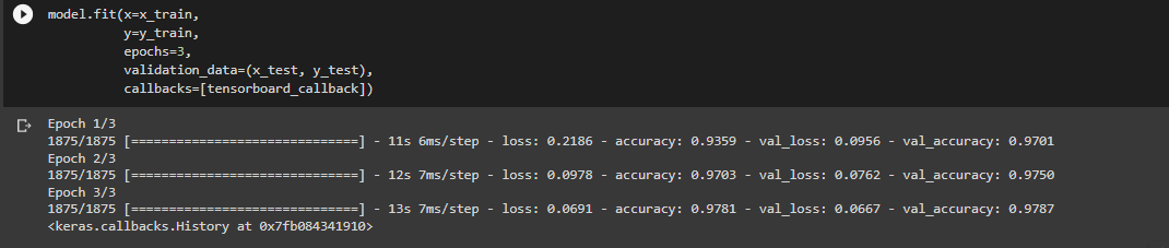
- Finally, train (or fit) the machine learning model on three epochs (iterations).
model.fit(x=x_train,
          y=y_train,
          epochs=3,
          validation_data=(x_test, y_test),
          callbacks=[tensorboard_callback])
Step 3 – How to Evaluate the Model
To start TensorBoard within your notebook, run the code below:
%tensorboard --logdir logs/fit
You can now view the dashboards showing the metrics for the model on tabs at the top and evaluate and improve your machine learning models accordingly.
Step 4 – How to Improve the Model
Since the point of evaluating your Machine Learning models is to gain better insight to improve the algorithm, it is imperative that we enhance our model. With these visuals, you can now see the in-depth performance of the model.
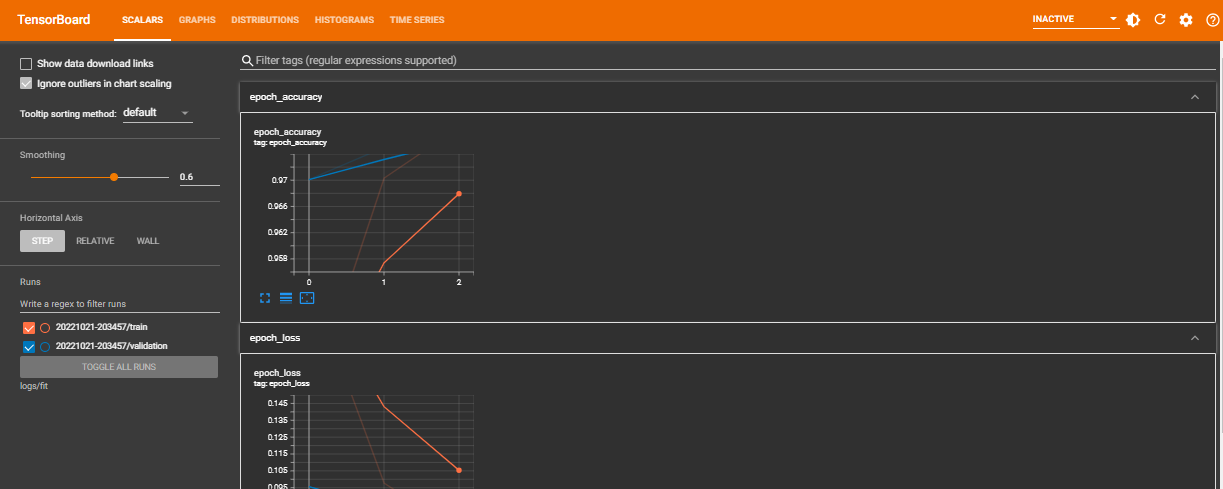
- The
Scalarsdashboard can be used to observe other scalar values such as training efficiency and learning rate. It demonstrates how the metrics and loss fluctuate with each epoch. - As the name implies, the
Graphsdashboard is used to visualize your model.
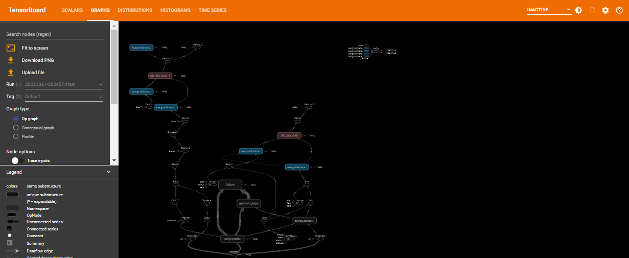 The Graph with the tensorboard
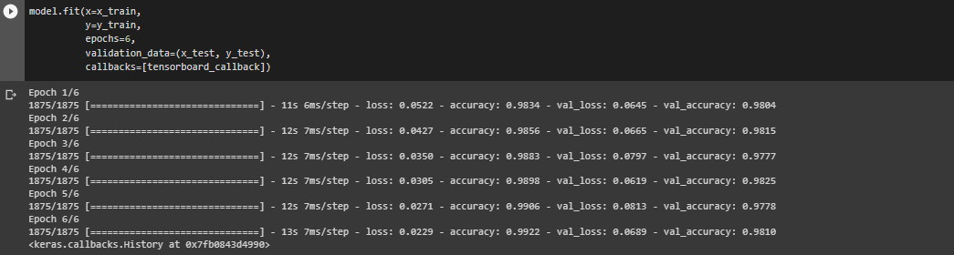
To improve this model, you will adjust the number of epochs from 3 to 6 and see how the model performs.
In general, the number of epochs is the number of iterations over the entire training dataset the machine learning model is trained on.
Intuitively, increasing this number almost always improves the performance of your machine learning model. To do this, you will run the code as follows:
model.fit(x=x_train,
          y=y_train,
          epochs=6,
          validation_data=(x_test, y_test),
          callbacks=[tensorboard_callback])
With the change we made, you can then generate another TensorBoard like this:
%tensorboard --logdir logs/fit
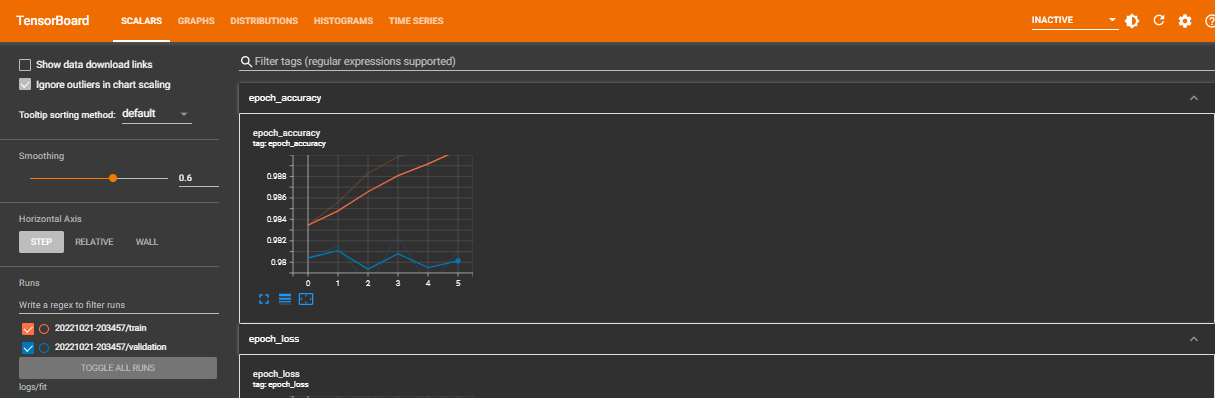
From the newly generated visuals, you can see that there is a remarkable improvement in the model's performance.
Conclusion
In this article, you learned how you can use TensorBoard to assess and improve your Machine Learning model's performance.
If at this point you have questions about the difference between TensorBoard and TensorFlow Metrics Analysis (TFMA), this is a valid concern. After all, both are tools for providing the measurements and visualizations needed during the Machine Learning workflow.
But it is important to note that you use each of these tools in distinct stages of the development process. At its core, TensorBoard is used to analyze the training process itself, while TFMA is concerned with the analysis of the 'finished' trained model.
Finally, I share my writings on Twitter if you enjoyed this article and want to see more.
Thank you for reading :)