How to Model an Epidemic with R

Epidemiology has never been more topical. It is the scientific study of how health and disease affects populations, including infectious diseases such as COVID-19.

Key to understanding the spread of such diseases is the practice of epidemic modeling. This involves building quantitative models to describe and forecast the spread of disease.

The classical approach to epidemic modeling is to use a type of mathematical model known as a "compartmental model".

The approach is as follows:

Assign each individual in the population to one of several compartments, based on their infection status.
Then, define the rates at which individuals move between compartments as their status updates.
Use this model to define differential equations that can predict the course of the epidemic.

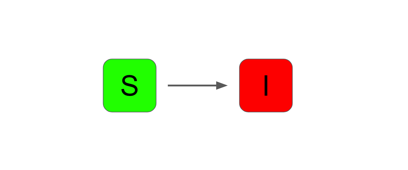
The SI model is the most basic form of compartmental model. It has two compartments: "susceptible" and "infectious".

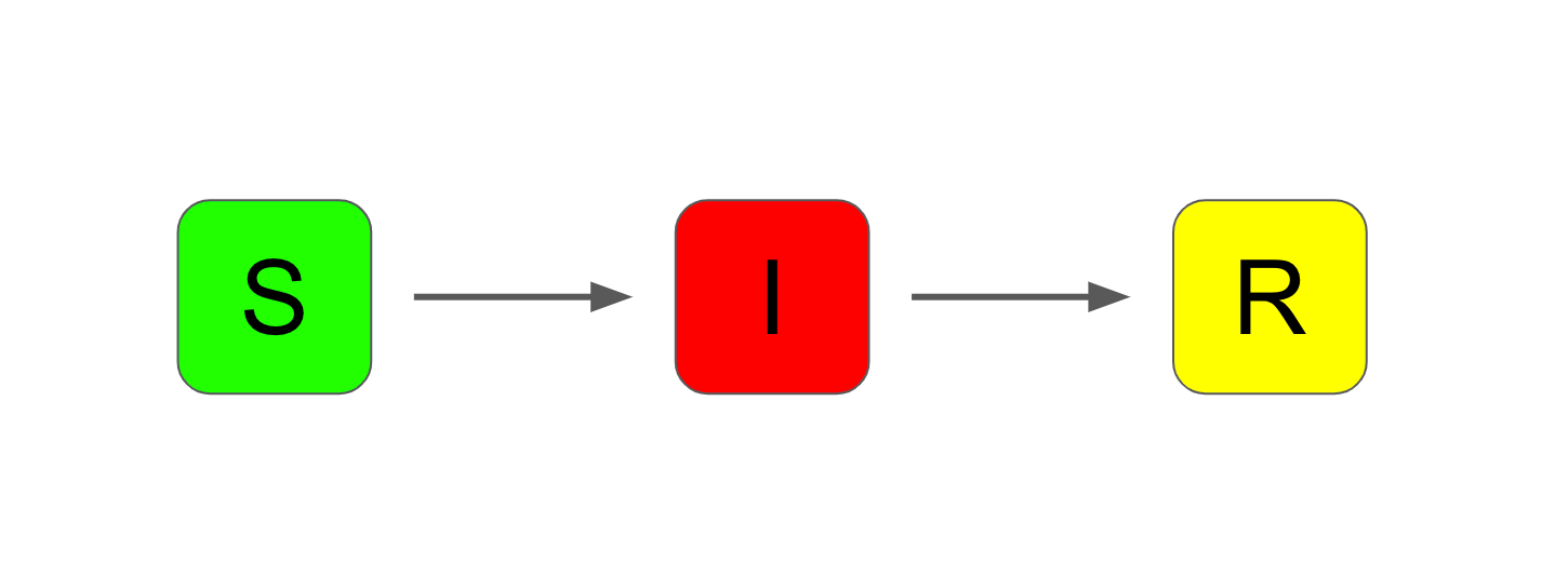
Two compartments, one labelled S, the other I. An arrow flows from S into I.

The SIR model adds an extra compartment called "recovered". This model is often used as a baseline in epidemiology. It is a simplistic model that nevertheless characterises the progression of an epidemic reasonably well.

Three compartments, labelled S, I and R. Arrows flow from S to I and from I to R.

An extension to the SIR model (and the one we will consider in more detail in this article) is the SEIR model. This adds one more compartment – "exposed".

What is the SEIR model?

The basic SEIR model has four compartments:

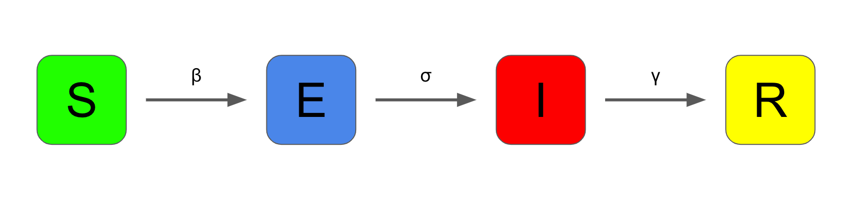
Four compartments. S flows into E, E flows into I, I flows into R. The three arrows are labelled beta, sigma and gamma respectively.

"Susceptible" – individuals who have not been exposed to the virus
"Exposed" – individuals exposed to the virus, but not yet infectious
"Infectious" – exposed individuals who go on to become infectious
"Recovered" – infectious individuals who recover and become immune to the virus

The population size N is taken as the sum of the individuals in the four compartments.

The flow of individuals between compartments is characterised by a number of parameters.

β - "beta"

β is the transmission coefficient. Think of this as the average number of infectious contacts an infectious individual in the population makes each time period. A high value of β means the virus has more opportunity to spread.

σ - "sigma"

σ is the rate at which exposed individuals become infectious. Think of it as the reciprocal of the average time it takes to become infectious. That is, if an individual becomes infectious after 4 days on average, σ will be 1/4 (or 0.25).

γ - "gamma"

γ is the rate at which infectious individuals recover. As before, think of it as the reciprocal of the average time it takes to recover. That is, if it takes 10 days on average to recover, γ will be 1/10 (or 0.1).

μ - "mu"

μ is an optional parameter to describe the mortality rate of infectious individuals. The higher μ is, the more deadly the virus.

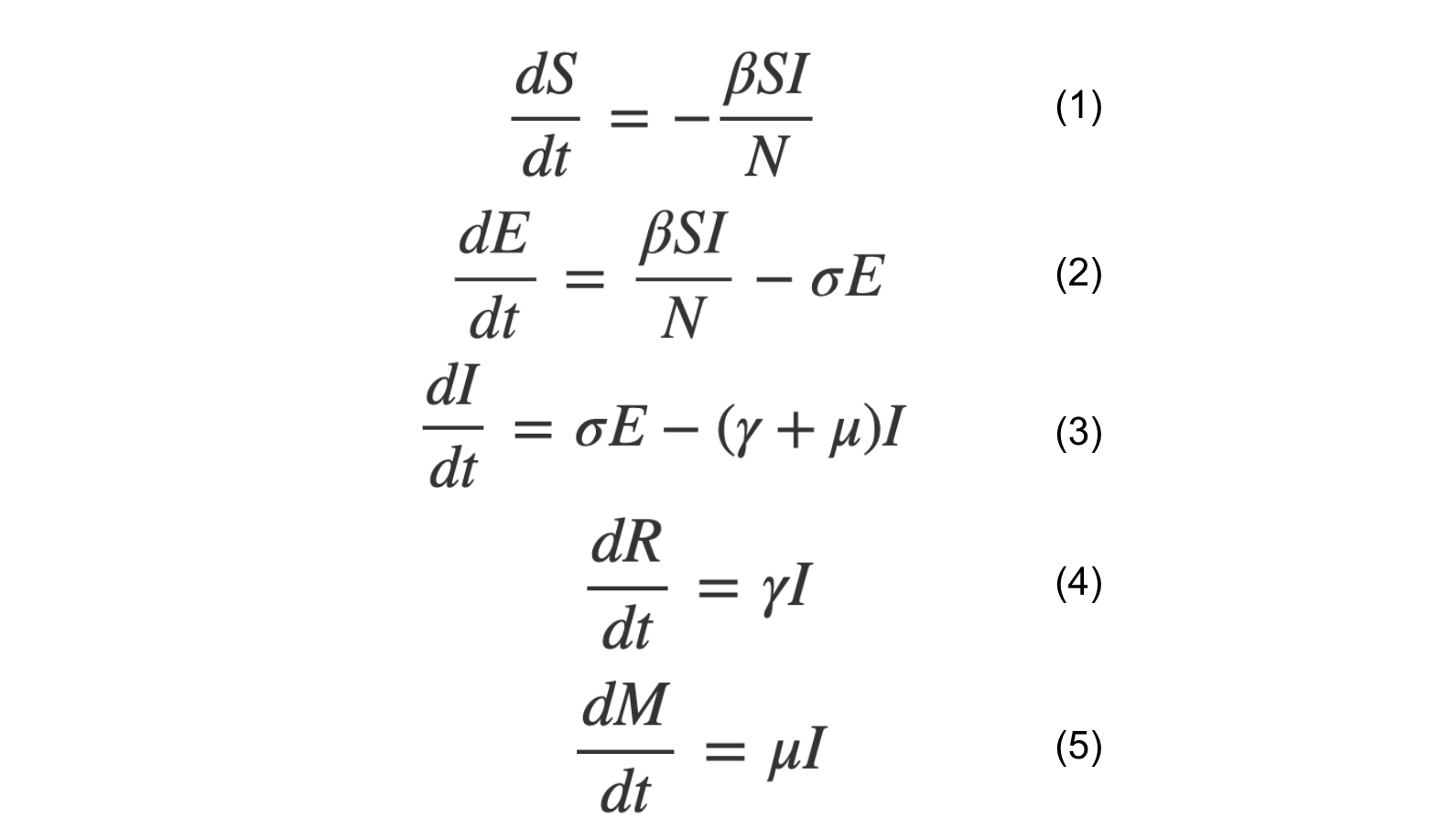
From these parameters, you can construct a set of differential equations. These describe the rate at which each compartment changes size.

Let's start with the "susceptible" compartment, S.

Equation (1) - Susceptible

The first thing to see from the model is that there is no way S can increase over time. There are no flows back into the compartment. Equation (1) must be negative, as S can only ever decrease.

In what ways can an individual leave compartment S?

Well, they can become infected by an infectious individual in the population.

At any stage, the proportion of infectious individuals in the population = I/N.

And the proportion of susceptible individuals will be S/N.

Under the assumption of perfect mixing (that is, individuals are equally likely to come into contact with any other in the population), the probability of any given contact being between an infectious and susceptible individual is (I / N) * (S / N).

This is multiplied by the number of contacts in the population. This is found by multiplying the transmission coefficient β, by the population size N.

Combining that all together and simplifying gives equation (1):

delta S equals minus beta times S times I all over N

Equation (2) - Exposed

Next, let's consider the "exposed" compartment, E. Individuals can flow into and out of this compartment.

The flow into E will be matched by the flow out of S. So the first part of the next equation will simply be the opposite of the previous term.

Individuals can leave E by moving into the infectious compartment. This happens at a rate determined by two variables – the rate σ and the current number of individuals in E.

So overall equation (2) is:

deltaEI equals beta times S times I all over N, subtract sigma times I

Equation (3) - Infectious

The next compartment to consider is the "infectious" compartment, I.

There is one way into this compartment, which is from the "exposed" compartment.

There are two ways an individual can leave the "infectious" compartment.

Some will move to "recovered". This happens at a rate γ.

Others will not survive the infection. They can be modeled using the mortality rate μ.

So equation (3) looks like:

delta I equals sigma times E subtract gamma times I subtract mu times I

Equation (4) - Recovered

Now let's look at the "recovered" compartment, R.

This time, individuals can flow into the compartment (determined by the rate γ).

And no individuals can flow out of the compartment (although in some models, it is assumed possible to move back into the "susceptible" compartment).

So the overall equation (4) looks like this:

Equation (5) - Mortality (optional)

Using similar reasoning, you could also construct equation (5) for the change in mortality. You might consider this a fifth compartment in the model.

If you set μ to zero, you can exclude this aspect of the model.

So now you have the full set of differential equations (1-5).

An important number in any epidemic model is known as the basic reproduction number, or R₀. This is defined as:

This number estimates the number of people who will be infected by the average infectious individual.

Therefore, it is a crucial number:

If R₀ is above 1, then an outbreak of the virus is likely to become an epidemic
If R₀ is below 1, then an outbreak is likely to be contained

How to solve these equations

In order to use the model to predict the course of the epidemic, it is necessary to solve the system of equations.

This can be done using the R programming language.

In particular, you can use a package called deSolve to solve the differential equations with respect to a time variable.

In R, paste the following code:

require(deSolve)

SEIR <- function(time, current_state, params){
  
  with(as.list(c(current_state, params)),{
    N <- S+E+I+R
    dS <- -(beta*S*I)/N
    dE <- (beta*S*I)/N - sigma*E
    dI <- sigma*E - gamma*I - mu*I
    dR <- gamma*I
    dM <- mu*I
    
    return(list(c(dS, dE, dI, dR, dM)))
  })
}

This code imports the deSolve package.

It then defines a function called SEIR. It takes three arguments:

The current time step.
A list of the current states of the system (that is, the estimates for each of S, E, I and R at the current time step).
A list of parameters used in the equations (recall these are β, σ, γ and μ).

Inside the function body, you define the system of differential equations as described above. These are evaluated for the given time step and are returned as a list. The order in which they are returned must match the order in which you provide the current states.

Now take a look at the code below:

params <- c(beta=0.5, sigma=0.25, gamma=0.2, mu=0.001)

initial_state <- c(S=999999, E=1, I=0, R=0, M=0)

times <- 0:365

This initialises the parameters and initial state (starting conditions) for the model.

It also generates a vector of times from zero to 365 days.

Now, create the model:

model <- ode(initial_state, times, SEIR, params)

This uses deSolve's ode() function to solve the equations with respect to time.

See here for the documentation.

The arguments required are:

The initial state for each of the compartments
The vector of times (this example solves for up to 365 days)
The SEIR() function, which defines the system of equations
A vector of parameters to pass to the SEIR() function

Running:

summary(model)

...will give the summary statistics of the model.

               S            E            I         R         M
Min.    108263.6 3.616607e-07 0.000000e+00      0.00    0.0000
1st Qu. 108263.7 5.957435e-03 1.414971e-02  63894.43  319.4721
Median  108395.7 8.470071e+00 1.273726e+01 886814.36 4434.0718
Mean    362798.6 9.745754e+03 1.212158e+04 612272.74 3061.3637
3rd Qu. 852375.5 1.734331e+03 2.533956e+03 887299.83 4436.4991
Max.    999999.0 1.092967e+05 1.265161e+05 887299.86 4436.4993
N          366.0 3.660000e+02 3.660000e+02    366.00  366.0000
sd      381257.2 2.475783e+04 2.969234e+04 387333.47 1936.6673

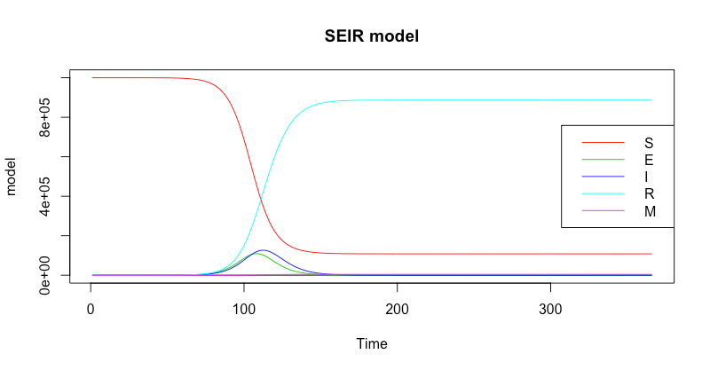
Already, you will find some interesting insights.

Out of a million individuals, 108,264 did not become infected.
At the peak of the epidemic, 126,516 individuals were infectious simultaneously.
887,300 individuals recovered by the end of the model.
A total of 4436 individuals died during the epidemic.

You can also visualise the evolution of the pandemic using the matplot() function.

Alternatively, you could use another plotting library such as ggplot2 to produce better quality graphics.

matplot(model, type="l", lty=1, main="SEIR model", xlab="Time")

legend <- colnames(model)[2:6]

legend("right", legend=legend, col=2:6, lty = 1)

The plot is shown below:

Chart showing curves which represent how the size of each compartment changes over time. S declines in a S-shaped curve, R and M increase in S-shape curves. I and E peak after day 100 before declining to zero

You can also coerce the model output to a dataframe type. Then, you can analyse the model further.

infections <- as.data.frame(model)$I

peak <- max(infections)

match(peak, infections)

The code above reveals that the number of infections peaked on day 112.

Using other libraries, such as dplyr, would let you carry out analysis as advanced as you'd like.

How to model intervention methods

The SEIR model is an interesting example of how an epidemic develops without any changes in the population's behaviour.

You can build more sophisticated models by taking the SEIR model as a starting point and adding extra features.

This lets you model changes in behaviour (either voluntary or as a result of government intervention).

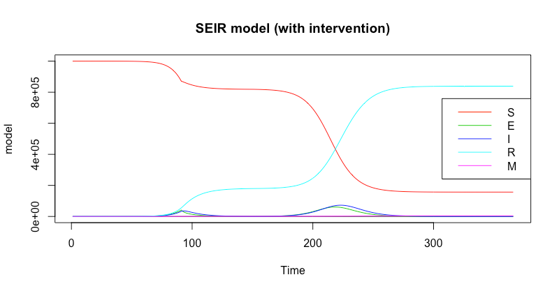
Many (but not all) countries around the world entered some form of "lockdown" during the coronavirus pandemic of 2020.

Ultimately, the intention of locking down is to alter the course of the epidemic by reducing the transmission coefficient, β.

The code below defines a model which changes the value of β between the start and end of a period of lockdown.

All the numbers used are purely illustrative. You could make an entire research career (several times over) trying to figure out the most realistic values.

SEIR_lockdown <- function(time, current_state, params){
  
    with(as.list(c(current_state, params)),{
      
      beta = ifelse(
        (time <= start_lockdown || time >= end_lockdown),
        0.5, 0.1
        )
      
      N <- S+E+I+R
      dS <- -(beta*S*I)/N
      dE <- (beta*S*I)/N - sigma*E
      dI <- sigma*E - gamma*I - mu*I
      dR <- gamma*I
      dM <- mu*I
      
      return(list(c(dS, dE, dI, dR, dM)))
    })
  }

The only change is the extra ifelse() statement to adjust the value of β to 0.1 during lockdown.

You need to pass two new parameters to the model. These are the start and end times of the lockdown period.

Here, the lockdown begins on day 90, and ends on day 150.

params <- c(
    sigma=0.25,
    gamma=0.2,
    mu=0.001,
    start_lockdown=90,
    end_lockdown=150
    )
  
  initial_state <- c(S=999999, E=1, I=0, R=0, M=0)
  
  times <- 0:365
  
  model <- ode(initial_state, times, SEIR_lockdown, params)

Now you can view the summary and graphs associated with this model.

summary(model)

This will reveal:

               S            E           I         R         M
Min.    156885.7 7.699207e-01     0.00000      0.00    0.0000
1st Qu. 160478.2 6.929205e+01    97.71405  63668.75  318.3438
Median  789214.4 1.246389e+03  1735.66330 194379.16  971.8958
Mean    589558.9 9.216918e+03 11460.62036 387824.44 1939.1222
3rd Qu. 867639.6 1.030043e+04 13780.17591 829898.56 4149.4928
Max.    999999.0 6.083432e+04 72443.97892 838916.89 4194.5845
N          366.0 3.660000e+02   366.00000    366.00  366.0000
sd      350719.3 1.570278e+04 18893.31145 346542.57 1732.7128

You can see:

Out of a million individuals, 156,886 did not become infected.
At the peak of the epidemic, 72,444 individuals were infectious simultaneously.
838,917 individuals recovered by the end of the model.
A total of 4195 individuals died during the epidemic.

Plotting the model using matplot() reveals a strong "second wave" effect (as was seen across many countries in Europe towards the end of 2020).

  matplot(
    model, 
    type="l",
    lty=1, 
    main="SEIR model (with intervention)", 
    xlab="Time"
    )
    
legend <- colnames(model)[2:6]

legend("right", legend=legend, col=2:6, lty = 1)

Chart showing curves which represent how the size of each compartment changes over time. S declines rapidly, before levelling out during the lockdown, and then declining rapidly again, R and M increase rapidly before levelling out, then increasing rapidly again. I and E show a small peak before day 100, then declines, before peaking again after day 200

Finally, you can coerce the model to a dataframe and carry out more detailed analysis from there.

infections <- as.data.frame(model)$I

peak <- max(infections)

match(peak, infections)

In this scenario, the number of infections peaked on day 223.

In other scenarios, you could model the effect of vaccination. Or, you could build in seasonal differences in the transmission rate.

Limitations of compartmental models

As with all modeling, an epidemic model is only as good as the data and assumptions that go into it.

And some of the assumptions behind the SEIR model as described are unrealistic.

For example:

In large populations, mixing is non-uniform. Individuals are much more likely to interact with individuals in their locality. More advanced compartmental models will account for this.
The model assumes the population is isolated. In reality, mixing between populations allows a virus to be introduced and reintroduced multiple times.
Individuals are usually not born with immunity. More sophisticated models will factor in the birth rate when considering longer periods of time.
The basic SEIR model does not account for age structures in the population. Often, a virus will spread faster among younger, densely populated cities. But it might prove more deadly to older populations outside those cities. More complex models will take these differences into consideration.
The SEIR model considers only averages for each of its parameters. In reality, there will be a lot of variation. Some individuals remain infectious for a long time. A small number of individuals might make a very large number of contacts. Therefore, the model is suitable for describing the epidemic at a high level, over a long period of time. But it is not suitable for predicting details on a smaller scale.

Despite its limitations, the SEIR model is a solid starting point for understanding the dynamics of an epidemic.

More generally, the approach of using differential equations to represent flows between compartments to model complex processes is very powerful.

And the availability of software packages for languages such as R and Python makes it easier than ever to get started exploring these techniques.

You can dig into the code used for the examples here.

Thanks for reading!