by Nezar Assawiel

How to strategically accomplish your machine learning model’s performance goals

Introduction

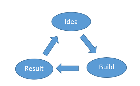
Machine learning (ML) development is an iterative process. You have an idea to solve the problem at hand, you build the idea and examine the results. You get another idea to improve the results and so on until you reach the performance goal that deems your model ready for deployment into production — ready to use by end users.

However, there are often many ideas and possibilities you can try to improve the performance and get closer to your goal. For example, you can collect more data, train longer, or try bigger or smaller networks.

Going in the wrong direction during this experimentation process can be costly, especially for large projects. No one wants to spend two months collecting more data to discover later on that the performance gain was negligible and it was not worth a day let alone two months!

Strategically setting and working towards the performance goal of your ML model is vital in speeding up the experimentation process and achieving that goal. In this post, I present some tips that will hopefully help you in this regard.

Expected prior knowledge

This post assumes knowing, at least, the basics of building a ML model. This discussion is not meant to illustrate what a ML model is or how to build one. Rather, the content is on how to strategically improve a ML model during the development process. Specifically, the following concepts and terminologies should be familiar to you:

• train, dev (development), and test sets: The dev set is also called the validation or the hold-on set. This post is a great short introduction to the topic.
• evaluation (or performance) metrics: Which are the measures used to indicate how “good” a ML model is in doing its job. Here is a post covering some of the basic metrics used in ML.
• bias (underfitting) and variance (overfitting) errors: This is great explanation of these errors in a simple way.

The importance of orthogonalization

As you know, the sequential steps in developing a ML model are as follows:

1. fit the training set well. For example try a bigger network, try another cost-function optimization method, try training longer.
2. fit the dev set well. For example try regularization, try collecting more training data.
3. fit the test set well. For example try a bigger dev set.
4. perform well in production. If not, the dev set needs to change or the cost function of the model.

During this process, ideally you would like the modifications you try — “model controls” — to be independent. Why?

Consider, for example, the steering wheel of a car. When you steer the wheel left, the car moves left. When you steer it right, the car moves right. What if steering the wheel left moved the car left and increased the speed of the car? It would become much more difficult to control the car, right? Why? Because steering the wheel left is not an independent control of the car any more. It is coupled with another control, the speed control. It is always easier when the controls are independent.

In ML development, early stopping, for example, is a form of regularization used to improve the performance on the dev set by training only on a part of the training set. So, early stopping is a control that is not independent from another control, namely how long you train.

For faster iterative development process, you would like the independence of your controls, that is, orthogonalization. In other words, consider avoiding dependent controls like early stopping as much as you can for faster development process.

Strategies

With the previous introduction in mind, here are some tips to set and strategically improve your model’s performance:

a) Combine multiple evaluation metrics into one

It is likely you have several evaluation metrics to evaluate the performance of your ML model. For example, you might have recall and precision to evaluate a classifier. Recall and precision are competing metrics — typically when one increases, the other decreases. So, how do you choose the best classifier from Table 1 below, for example?

It is a good idea in this case to combine precision and recall into one metric. The F1 score [F1 score= (2 *precision*recall)/(precision + recall)] will do, as you might have realized already. As such, Classifier A from Table 1 will have the best F1 score.

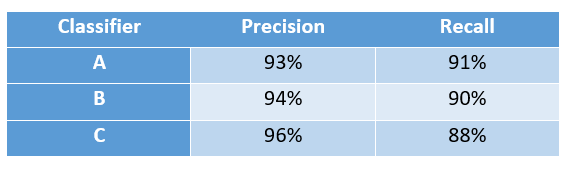
Obviously, this process is problem-specific. Your application might require maximizing precision. In this case, Classifier C in Table 1 will be your best choice.

Optimizing and satisficing

You might want to follow the optimizing and satisficing approach. Meaning, you are optimizing one metric as long as the other metric(s) meet a certain minimum threshold.

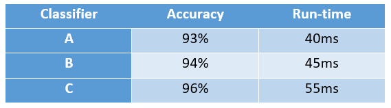
Assume the classifiers from Table 1, and accuracy and run-time as two metrics as shown in Table 2 below. You may be mainly concerned about optimizing one metric — accuracy — as long as the other metrics — run-time — meet a certain threshold. In this example, the run-time threshold is 50 ms or less. So, you are looking for the classifier with the highest accuracy as long as the run-time is 50 ms or less. Thus, from Table 2, you would choose Classifier B.

However, if your aim is to maximize the performance across all metrics, you would need to combine them.

It is not always easy to combine all metrics into one. There may be many of them. The relationship between them is not clear. In such cases, you would need to be creative and careful in combining them! The time you invest in coming up with an all-in-one performance metric is worth it. It won’t only speed up the development process, but will also produce a well-performing model in production.

b) Set the train, dev, and test sets correctly

Choose the right size for the train/dev /test split

You have likely seen the 60%, 20%, 20% split for the train, dev, test data sets, respectively. This works well for small data sets — say 10k data points or fewer. However, when working with large data sets, especially with deep learning, a 98%, 1%, 1% split or similar might be more appropriate. If you have 2 million data points in your dataset, a 1% split is 20K data points which are enough for the dev and test sets.

In general, you want your dev set to be large enough to capture the changes you make to your model during your experimentation process. You want your test set to be large enough to give you high confidence in the performance of your model.

Make sure the dev and test sets come from the same distribution

While this may seem trivial, I have seen experienced developers forget this important point. Say you have experimented and iteratively improved a model that predicts default on car loans based on zip code. Don’t expect your model to work correctly on a test set from zip code areas with low average-income if the dev set comes from zip code areas with high average-income, for example. These are two different distributions!

Make sure the dev and test sets reflect the data your model will encounter in production

For example, if you are doing face-recognition, the resolution of your dev/test images should reflect the resolution of the images in production. While this might be a trivial example, you should examine all aspects of the data on which your application would work in production in comparison to your train/dev/test data. If your model is doing well on your metric and dev/test sets but not so well in production, you have the wrong metric and/or the wrong dev/test sets!

c) Identify and tackle the “correct” error first

Bayes’ error and human error

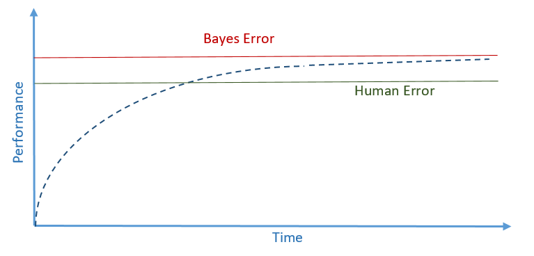
Bayes’ error is the theoretical lowest error that exists in a model, in other words irreducible error. Consider, for example, a dog classifier that predicts if the image at hand is of a dog or another animal. There might be some images that are so blurry that are impossible to classify by humans or even the most sophisticated system that has ever been invented. This will be Bayes’ error.

Human error, by definition, is larger — worse — than Bayes’ error. However, human error is usually very close to Bayes’ error since we are really good at recognizing patterns. Thus, human error is usually used as a proxy for Bayes error.

Improving below human-level performance

When the performance of your ML model is below human-level performance, you can improve the performance by:

1. getting more labeled data by humans
2. analyzing the errors and incorporating the insights into the system. Why does the ML model get this and that wrong while humans get them right?
3. improving the model itself. Look at whether it underfits — high bias error — or overfits — high variance error — and change the model accordingly.

Once human-level performance is surpassed, improving the performance becomes a much slower and more difficult process as you would expect.

So, how do you define human error exactly? This is what is discussed next!

Defining human error and identifying the error to tackle first

Consider the dog classification problem from before — recognizing if an image is of a dog or not. After doing some research, you might find the human error as follows:

• average person: 2% error
• average zoologist: 1% error
• expert zoologist: 0.6% error
• a team of expert zoologists: 0.4% error

Now, consider the four cases in Table 3 below.

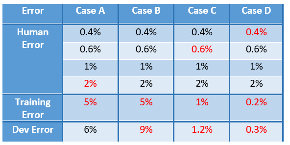
In Case A, your priority should be the underfitting problem — high bias — as indicated by the errors in red, since the bias error (5% -2% =3%) is larger than the variance error (6% -5% =1%). For the human error, the largest among the human errors that are smaller than the training error is used first. Thus, your human error reference in this case is that of the average person — 2% — since it is the largest error among the human errors that are smaller than the training error (all of them in this case).

In Case B, you might need to improve the variance error first, 9%-5%=4%, since it is larger than the bias error of 5%-2%=3%.

In Case C, you surpassed the human performance of the average person and you are tied to the performance of the average zoologist. So, your new human error should be that of the expert zoologist — 0.6% — or even the team of expert zoologists — 0.4%. The variance error in this case is 0.2% while the bias error is between 0.4% and 0.6%. So, you should work on this error first — need to better fit the training data.

Surpassing human performance

In Case D, you see that the training error is 0.2% while the best human error is 0.4%. Does this mean your model surpassed human performance or the model overfits by 0.2%?! You see, it is not clear whether to focus on the bias error or the variance error. Also, if, indeed, your model surpassed human performance and you are still looking to improve the model, it becomes unclear which strategy to follow from a human intuition perspective.

There are many ML models nowadays that surpass human performance, such as product recommendation and online-ad targeting systems. These “models that surpass human performance” tend to be non-natural perception systems, that is, not computer vision, speech recognition or natural language processing systems. The reason for this is that we humans are really good at natural perception tasks.

With big data and deep learning, however, there are natural perception systems that surpass human performance and they are getting better and better. But these are much harder problems than non-natural perception problems.

Originally published at assawiel.com/blog on March 24, 2018. Edited: Oct 4, 2018