By Thalles Silva
Faces are everywhere — from photos and videos on social media websites, to consumer security applications like the iPhone Xs FaceID.
In this context, computer vision, applied to faces, has many subareas. These include face detection, recognition, and tracking. Moreover, with the advance of Deep Learning, these solutions are getting more mature for commercial applications.
This post shows you, piece-by-piece, how to design and train your own Convolutional Neural Network (CNN) for face identification. Here, we propose a Tensorflow Eager implementation of Siamese DenseNets.
You can find the complete code here.
Siamese DenseNets
A Siamese CNN is a class of neural nets (NNs) that contains two or more identical network instances. The term identical refers to the fact that the two NNs share the same design configuration and, most important, their weights.
To understand DenseNets, we need to focus on two principal components of its architecture. These are the dense block and the transition layer.
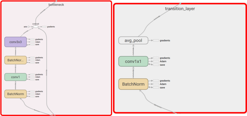
In short, a DenseNet is a stack of dense blocks followed by transition layers. A block consists of a series of units. Every unit packs two convolutions. Each convolution is preceded by batch normalization (BN) and rectified linear units (ReLU) activations.
Each unit outputs a fixed number of feature vectors. This number is controlled by a single parameter — the growth rate. Essentially, it manages how much new information a given unit allows to pass through to the next one.
Similarly, transition layers are simple components. They are designed to down-sample feature vectors passing through the network. Each transition layer consists of a BN operation, followed by a 1x1 convolution plus a 2x2average pooling.
The big difference from other regular CNNs is that each unit within a dense block is connected to every other unit before it. Within a block, the nth unit receives as input the feature-vectors learned by the n-1, n-2, … all the way down to the first unit in the pipeline. Put differently, the DenseNets design allows for high-level feature sharing among its units.
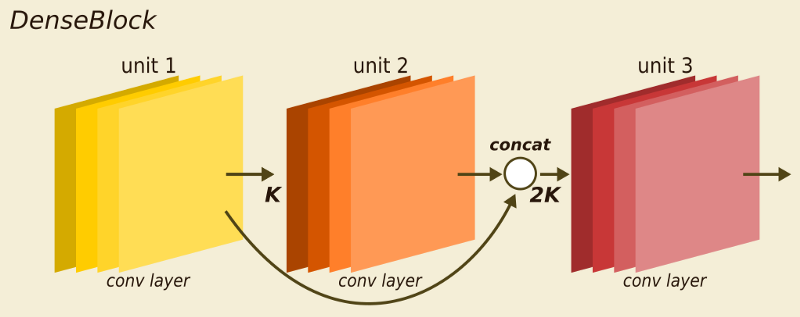 DenseBlock overview. Each unit outputs K feature vectors. The following units receive feature vectors from previous units by concatenation.
When compared to ResNets, DenseNets have feature reusing by concatenation instead of summation. As a consequence, DenseNets tend to be more compact in the number of parameters than ResNets. Intuitively, every feature-vector learned by any given DenseNet unit is reused by all the following units within a block. This minimizes the possibility of different layers of the network learning redundant features.
Both ResNets and DenseNets use the popular bottleneck layer design. It consists of 2 components:
- a 1x1 convolution to reduce the spatial dimensions of features
- a wider convolution, in this case a 3x3 operation for feature learning
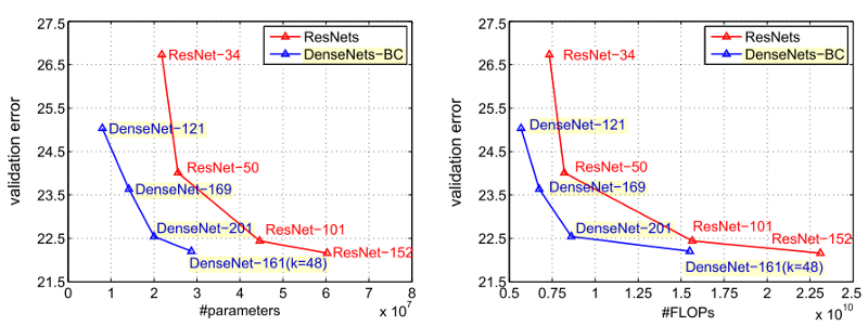
Regarding parameter efficiency and floating point operations per second (FLOPs), DenseNets surpass ResNets by a significant margin. DenseNets not only achieve smaller error rates on ImageNets, but also require fewer parameters and fewer FLOPs than ResNets.
Another trick that enhances model compactness is the compression factor. This procedure takes place on the transition layers and aims to reduce the number of feature vectors that go into the next dense block. DenseNets implement this mechanism by setting a factor, θ, between 0 and 1. θ controls how many of the current features are allowed to pass through to the following block. This technique allows DenseNets even more reduction in the number of feature-vectors, and to be very parameter efficient.
Learning face similarities
This is not a classification task — we do not want to categorize images into classes. Instead, we want to learn a representation that can individually describe each input.
Specifically, we want to find similarities between input images. To do that, we need a representation capable of expressing a relationship between two comparable things.
In practice, we want to learn embedding vectors to represent relationships among people’s face images. We want vectors with the following properties:
- If two images (X1 and X2) are similar, we want the distance between the 2 output vectors to be as small as possible
- If X1 and X2 are not similar, we want this distance to be as large as we can make it
Below we represent the whole Siamese DenseNets framework for learning face embeddings. The next sections go over the specific building blocks of this architecture.
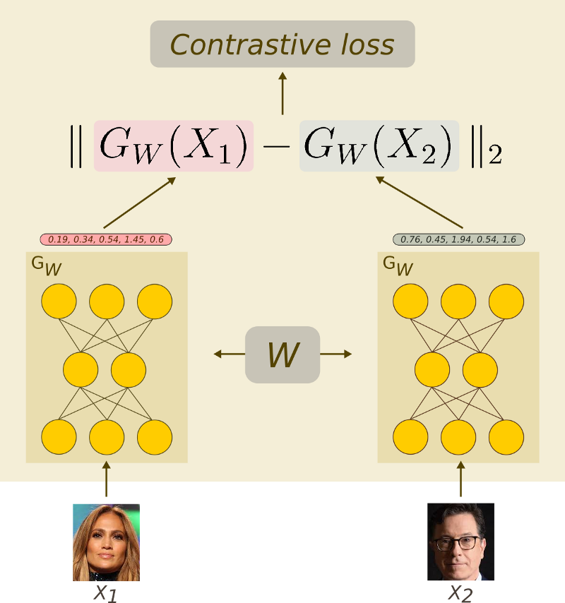
The contrastive loss
To understand how the contrastive loss works, the first thing to keep in mind is that it works on pairs of images.
Take the two images above as an example. At a given point, we give the pair (X1, X2) to the system with the following properties:
- if X1 is considered to be similar to X2 we give it a label of 0
- otherwise X1 gets a label of 1
Now, let’s define Gw as a parametric function — a neural network. Its role is very simple, Gw maps high-resolution input to low-resolution outputs.
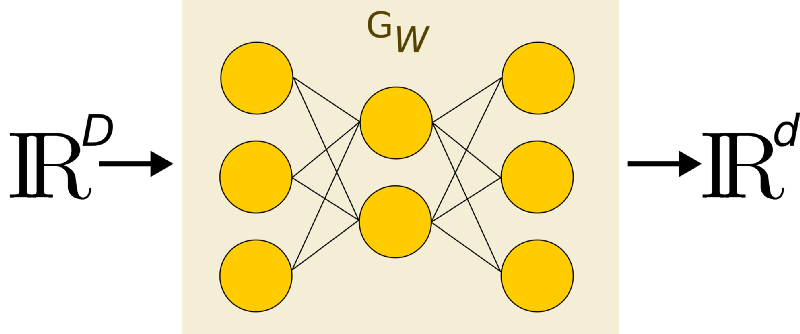 Reducing high dimensional input to a low dimensional representation (D < d)
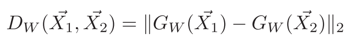
We want to learn a parameterized distance function Dw, between the inputs X1 and X2. This is the Euclidean distance between the outputs of Gw.
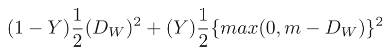
Note that m is the margin. It defines the radius around Gw. It controls how dissimilar images contribute to the total loss function. That is, a pair of images (X1, X2) from different people (class) only contribute to the loss if the distance between them is within the margin — if (m -Dw) > 0.
In other words, we want to optimize the system such that:
- If the pair of images is similar (label 0) we minimize the distance function Dw.
- If the pair of images is not similar (label 1), we increase the distance function Dw.
The final loss function and its implementation in Tensorflow are defined as follows:
It is important to note how we calculate the distance in line 2. Since this loss function has to be differentiable with respect to the model’s weights, we need to ensure that negative side effects will not take place.
Note that in the square root part of the equation, we add a small epsilon before computing the square root. And the reason is very subtle. In the case where the content inside the square root is zero, the square root of 0 is also 0 — which is fine.
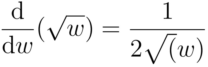 At w=0, the derivative of the sqrt() ope would result in a divide by 0. This would break your code or result in a NaN in python.
Yet, if the content is 0 and we are calculating the gradients, the derivative of the square root would have a divide by 0 operation. That is bad.
As a take-away, always make sure the routines you are using are computationally safe.
Moreover, when minimizing the contrastive loss using Stochastic Gradient Descent (SGD), there are two possible scenarios.
First, if the pair of input samples (X1, X2) is of the same class (label 0), the second part of the equation is zeroed-out. In this situation, we only minimize the distance between the two images of the same class. In practice, we are pushing the two representations to be as close to each other as possible.
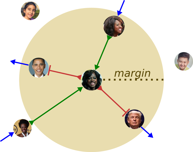 The Contrastive loss clusters similar faces together (inside a given area) and pushes not similar samples apart.
In the second case, if the input pair (X1, X2) is not from the same class (label 1), the first part of the equation is canceled. Then, in the second term of the summation, two situations may occur.
First, if the distance between the two image pairs X1 and X2 is greater than m, nothing happens. Note that if Dw >; m, then the difference between them will also be negative. As a result, the derivative of the remaining function will be 0 — no gradient equals no learning.
However, if the distance Dw between the input pair X1 and X2 is less than m, the opposite situation occurs. Now the gradient signal will act as a repulsive force. In practice, it will push the two representations farther away from one another.
Dataset
To train a Siamese CNN for face similarity we used the popular Large-scale CelebFaces Attributes (CelebA) dataset. It contains more than 200k celebrity images from 10,177 different identities. To ease the data pre-processing, we chose the aligned and cropped faces part of dataset. The following picture shows some of the dataset samples.
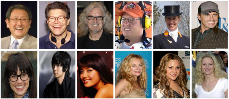 CelebA sample images.
To use the contrastive loss, we need to build the dataset in a very specific way. Basically, we need to build a dataset that contains a lot of face image pairs. Some of them from the same people, some of them from different ones.
To put it simply, given an input image Xi we need to find a set of sample S = {X1, X2,…,Xj} such that Xi and Xj belong to the same class. Put it another way, Xi and Xj are face images of the same person.
In the same way, we need to find a set of pictures D = {S1, S2,…,Sj} such that Sj does NOT belong to the same class as Xi.
Finally, we combine the input image Xi with samples from both similar and dissimilar sets. For every pair (Xi, Xj) if Xj belongs to the set of similar samples S, we assign a label of 0 to the pair, otherwise, it gets a label of 1.
Training Details
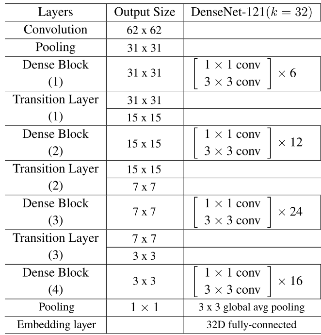
We used the DenseNet-121 design as described in the original paper. The growth rate parameter (k) was set to 32. Instead of the 1000D fully-connected layer at the end, we learn embedding vectors of size 32.
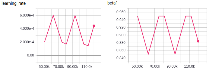
To optimize the model parameters, we used the Adam Optimizer with a cyclical learning rate schedule. Inspired by fast.ai super-convergence, we fixed the beta2 Adam parameter as 0.99 and applied a cycle policy to beta1.
In this way, both parameters:— the learning rate and beta1 — vary cyclically between a maximum and minimum value. Simply put, while the learning rate increases the beta1 decreases in a fixed interval.
Results
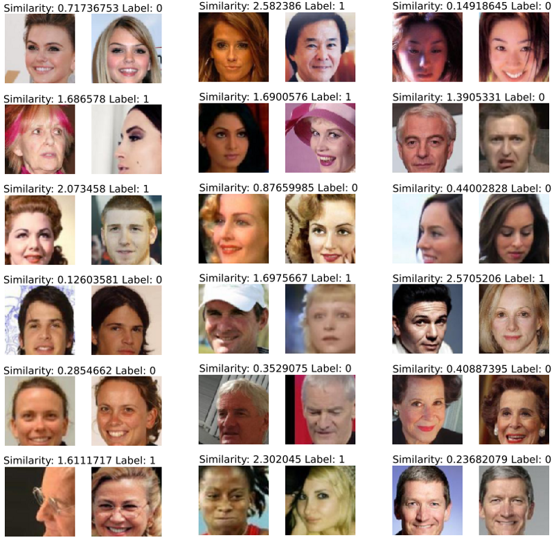
The results are very good.
For these examples, a single threshold of 1 would correctly classify most of the samples. Also, the network is invariant to many transformations of the input images. These transformations include variations of brightness and contrast, the size of the face, pose, and alignment. It is invariant to small changes in peoples looks such as age, haircut, hats, and glasses.
The similarity value below is smaller for similar faces and higher for dissimilar ones. Labels of 0 means that the pair of images are from the same person.
Thanks for reading!
For more cool stuff on deep learning, check out
Dive head first into advanced GANs: exploring self-attention and spectral norm
_Lately, Generative Models are drawing a lot of attention. Much of that comes from Generative Adversarial Networks…_medium.freecodecamp.orgDiving into Deep Convolutional Semantic Segmentation Networks and Deeplab_V3
_Deep Convolutional Neural Networks (DCNNs) have achieved remarkable success in various Computer Vision applications…_medium.freecodecamp.org