
A radiologist can mark a tumor on a CT scan by drawing a straight line across it. Creating a complete 3D segmentation requires outlining the tumor across the slices where it appears, which is more time-consuming.
This tutorial explains how Lumina works. It's a system that uses a CT scan and one RECIST line to produce a 3D segmentation mask of the marked tumor.
Lumina was developed for the FLARE 2026 pan-cancer segmentation challenge. The system was designed to run on a CPU with an 8 GB memory limit and a 60-second inference limit.
This tutorial covers the main design decisions, implementation details, and experiments that shaped the final system.
What We'll Cover:
Step 5: Use a Loss Function That Includes Boundary Information
Step 6: Transform the Probability Map into a Segmentation Mask
What Lumina Does
A radiologist can measure a tumor by drawing a line across its longest visible diameter. This is a RECIST measurement (Response Evaluation Criteria in Solid Tumors), which is widely used to measure tumor response during cancer treatment.
A RECIST line measures a 2D diameter marker. It doesn't describe the tumor's full 3D shape.
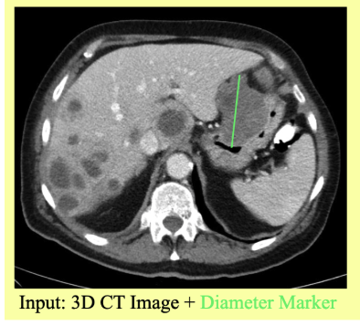
Lumina uses this measurement to prompt a 3D segmentation model.
The task can be described as:
Input: A 3D CT scan and a 2D RECIST line marking one tumor.
Output: A 3D mask of that tumor, with one label for each voxel.
A voxel is the 3D equivalent of a pixel. Each voxel represents a small volume of tissue in the CT scan.
The RECIST line tells the model which tumor to segment. The model then predicts the tumor's three-dimensional extent.
This makes the segmentation problem more specific because the model doesn't need to identify every possible tumor in the scan.
Lumina Pipeline Overview
The complete process has several stages. We start with a 3D CT scan and a RECIST line marking one tumor. We then convert the line into additional input channels, crop and resample the image, and pass the three channels through a 3D segmentation network.
The network produces a probability map, which we convert into the final 3D tumor mask through resampling, thresholding, and connected-component selection.
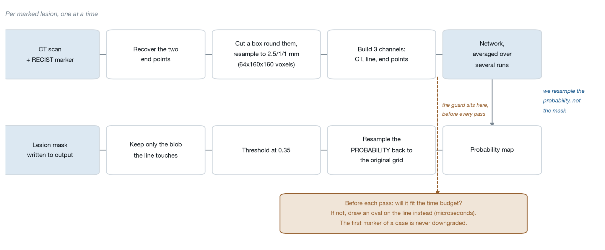
The main stages are:
Prepare the CT scan and RECIST marker.
Encode the RECIST line as additional network input.
Crop and resample the image to a common grid.
Predict the tumor probability map with a 3D segmentation network.
Refine the probability map and convert it into a binary mask.
Control CPU inference so the full case stays within runtime and memory limits.
Prerequisites
You'll get more from this tutorial if you have some experience with:
Python
NumPy
PyTorch
Basic convolutional neural networks.
No detailed medical background is required. The tutorial explains medical imaging concepts as it introduces them.
The implementation uses NumPy, SciPy, PyTorch, and MONAI, a medical imaging framework built on PyTorch.
Step 1: Review Your Data Before Coding
Our data was provided as .npz files, which is NumPy's compressed array format.
Each file contains fields similar to these:
imgs       # the CT scan, a 3D array
recist     # the marker lines, same shape, one integer per tumour
spacing    # how many millimetres apart the voxels are
origin     # where the scan sits in the scanner's coordinates
direction  # how the scan is rotated
gts        # the ground-truth segmentation, training files only
Before building the model, we inspected the image values, array shapes, and spatial metadata.
Two details were especially significant.
The Scans Were Already Brightness-Adjusted
CT scanners normally store images in Hounsfield units. Water is about 0 HU, while bone can exceed 1000 HU.
In this dataset, the scans had already been converted to a fixed 0–255 range. The original Hounsfield-unit values weren't available.
This meant that we couldn't apply the usual CT windowing process to the original values. Instead, we measured the intensity distribution of the data provided.
For example, 53.4% of the voxels had a value of exactly 0, corresponding to air outside the body.
Coordinate Order Matters
The spacing array is stored as (X, Y, Z), while NumPy arrays are indexed as (Z, Y, X).
If you mix these two conventions, spatial measurements can be incorrect.
We converted the coordinates once at the input boundary and used the (Z, Y, X) convention internally:
def _to_zyx(vec3, order):
    vec3 = np.asarray(vec3, dtype=float).ravel()
    if order == "xyz":
        return vec3[::-1].copy()      # (x, y, z) -> (z, y, x)
    if order == "zyx":
        return vec3.copy()
    raise ValueError(f"unknown geometry_order {order!r}")
The important lesson is to inspect several files before designing the preprocessing pipeline.
Check:
Array shapes
Intensity ranges
Voxel spacing
Coordinate conventions
Metadata
Available labels
Avoid assuming the data follows conventions from another CT dataset or tutorial.
Step 2: Turn the RECIST Line into Network Input
A neural network receives a stack of input channels. The CT scan provides the first channel. We then represent the RECIST line in a form the network can use.
We use three channels:
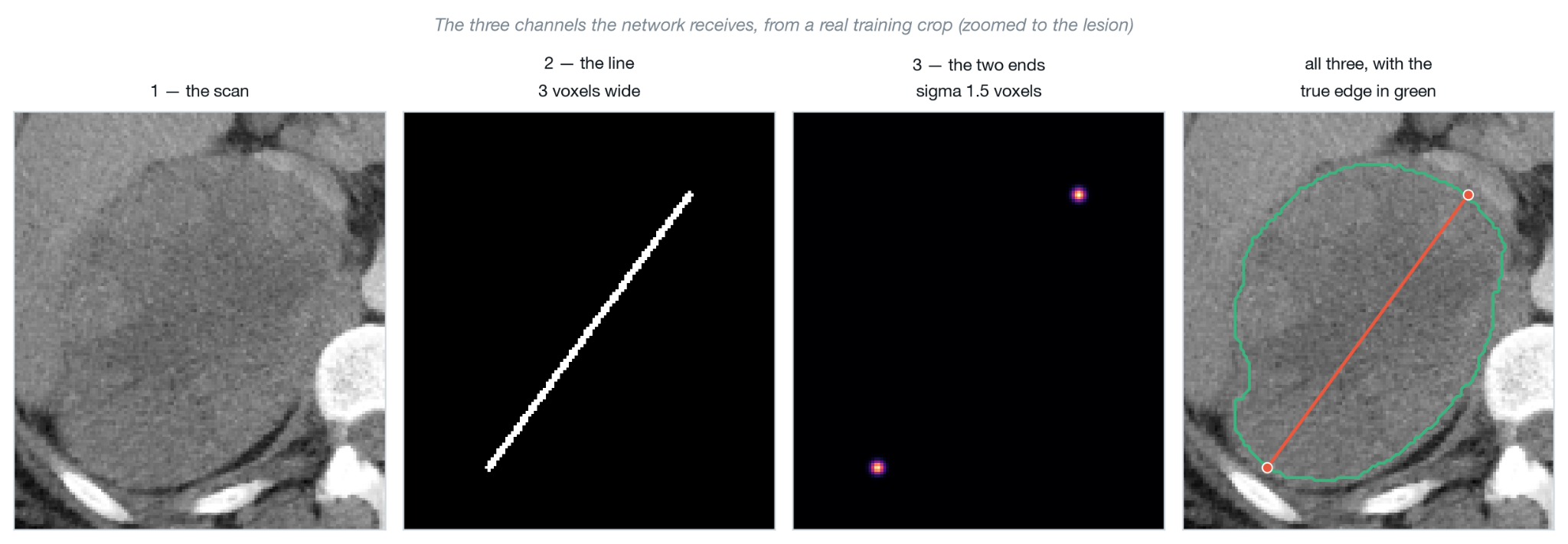
CT scan
RECIST line, drawn 3 voxels thick
Endpoint heatmap, containing a Gaussian around each endpoint
The two endpoints define the measured diameter and provide the network with the location and length of the RECIST measurement.
The endpoint information is represented using Gaussian functions. Each Gaussian has a high value near the endpoint and gradually decreases with distance.
def _endpoint_heatmap(endpoints_zyx, shape, sigma):
    d, h, w = (int(s) for s in shape)
    heat = np.zeros((d, h, w), dtype=np.float32)

    rad = max(1, int(np.ceil(3 * sigma)))
    two_s2 = 2.0 * sigma * sigma

    for z0, y0, x0 in np.asarray(endpoints_zyx, float):
        zc, yc, xc = int(round(z0)), int(round(y0)), int(round(x0)))

        zl, zr = max(0, zc - rad), min(d, zc + rad + 1)
        yl, yr = max(0, yc - rad), min(h, yc + rad + 1)
        xl, xr = max(0, xc - rad), min(w, xc + rad + 1)

        zz, yy, xx = np.mgrid[
            zl:zr, yl:yr, xl:xr
        ].astype(np.float32)

        g = np.exp(
            -((zz-z0)**2 + (yy-y0)**2 + (xx-x0)**2) / two_s2
        )

        np.maximum(
            heat[zl:zr, yl:yr, xl:xr],
            g,
            out=heat[zl:zr, yl:yr, xl:xr]
        )

    return heat
The Gaussian is calculated only in a small region around each endpoint.
With sigma = 1.5, values become very small several voxels away from the endpoint. Calculating the Gaussian over the complete volume would therefore perform unnecessary work.
Draw the Line at the Required Resolution
We also redraw the RECIST line from its two endpoints at the resolution the network requires.
We don't create the line at one resolution and then resize it with the image. Resizing a thin line can make it thinner or cause it to disconnect. Recreating the line from its endpoints keeps the prompt consistent with the image resolution.
Step 3: Align All Tumors on a Common Grid
CT scans can have different voxel spacings.
For example, one scan may have thin slices while another may have much thicker slices. The physical size represented by the same number of voxels can therefore vary between scans.
For each marked tumor, we'll create a fixed-size crop and resample it to a fixed voxel spacing.
Our configuration is:
target_spacing: [2.5, 1.0, 1.0]     # mm per voxel: z, y, x
crop_size:      [64, 160, 160]      # voxels: z, y, x
The in-plane dimensions correspond to a physical field of view of:
160 × 160 mm
The network therefore receives a consistent 64 × 160 × 160 input.
We use a target spacing derived from the training data. The 2.5 mm slice spacing was close to the median slice spacing in the training set.
We use a 160 mm crop based on the distribution of lesion sizes in the training data. It covers the 99th percentile of lesion extent.
Intensity Normalization
We also normalize the CT intensity values using statistics calculated from the training crops:
intensity_mean: 96.88
intensity_std: 79.00
The normalization is:
image = (image - 96.88) / 79.00
We calculate these statistics using only the training data.
We use the same values for validation and test data. We don't recalculate these statistics from the validation or test sets, because that would allow information from those sets to influence preprocessing.
For Lumina, the training-data statistics are a mean of 96.88 and a standard deviation of 79.00. We store these values in the configuration and use the same preprocessing during training, validation, and inference.
Step 4: Build the 3D Segmentation Network
Here, we'll use DynUNet from MONAI.
DynUNet is a 3D U-Net architecture based on ideas from nnU-Net and supports configurable network depth, kernels, strides, and residual connections.
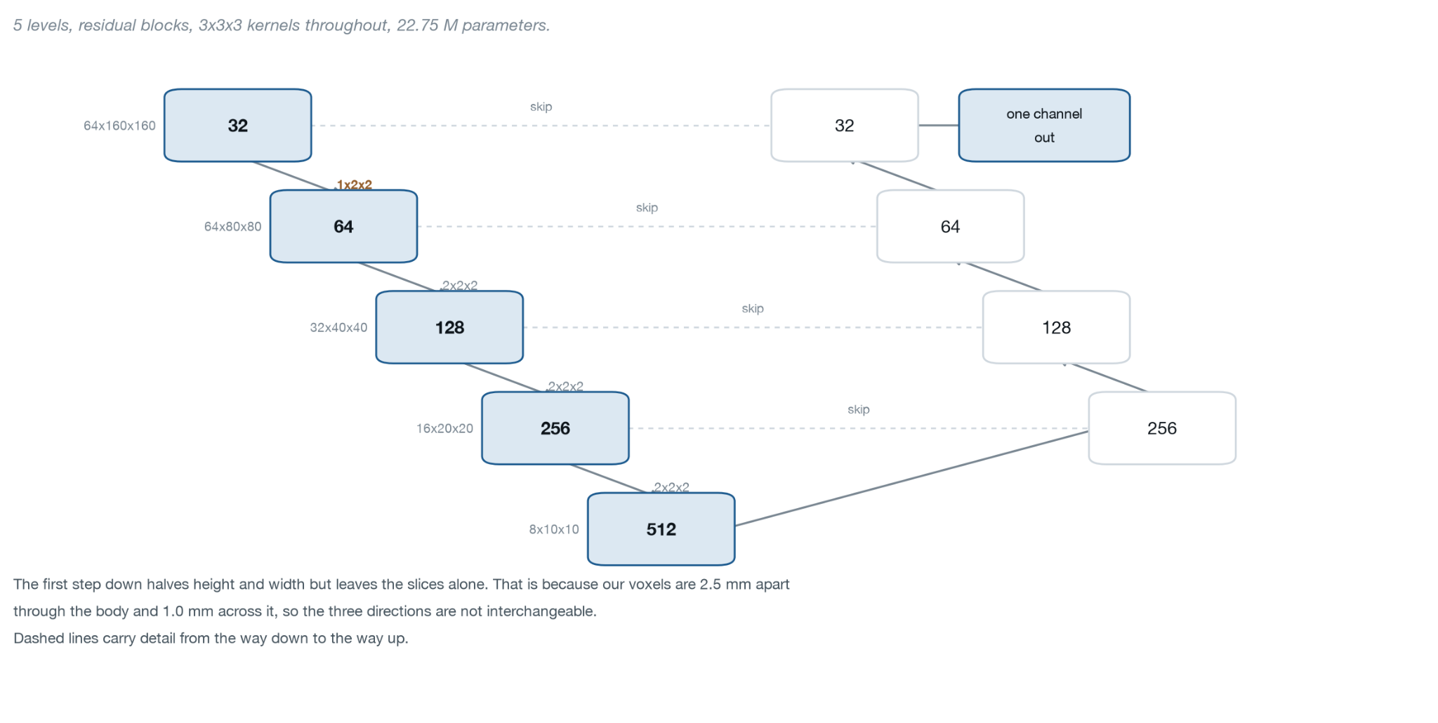
A U-Net has two main parts.
The encoder gradually reduces the spatial resolution while learning increasingly high-level features.
The decoder then restores the spatial resolution to produce a segmentation map.
Skip connections pass fine spatial details from the encoder to the decoder. This helps the decoder recover the tumor's boundary when it creates the final segmentation.
For Lumina, the network receives three channels:
CT
RECIST line
Endpoint heatmap.
The model configuration is:
from monai.networks.nets import DynUNet

# 5 levels; the first downsample skips z (see below).
kernels = [[3, 3, 3]] * 5
strides = [[1, 1, 1], [1, 2, 2], [2, 2, 2], [2, 2, 2], [2, 2, 2]]

model = DynUNet(
    spatial_dims=3,
    in_channels=3,          # CT + line + endpoint blobs
    out_channels=1,         # one probability per voxel
    kernel_size=kernels,
    strides=strides,
    upsample_kernel_size=strides[1:],
    filters=features,
    res_block=True,
)
The strides list is an important part of the configuration. Our voxels have different sizes: they're 2.5 mm apart between slices but only 1.0 mm apart within each slice. If we reduce all three dimensions at every level, we lose inter-slice detail too quickly. We'll therefore keep the z dimension unchanged during the first downsampling step. This helps preserve useful information in all three directions.
Lumina's main design work focuses on input representation, preprocessing, training strategy, post-processing, and CPU inference behavior.
Step 5: Use a Loss Function That Includes Boundary Information
During training, the network needs a way to measure how different its prediction is from the ground-truth segmentation. This measurement is called a loss function. The network adjusts its weights to reduce this loss.
For Lumina, we combine two common losses: Dice loss and binary cross-entropy (BCE).
Dice Loss
Dice loss focuses on the overlap between the predicted tumor region and the ground-truth region.
It's useful when we want the overall size and shape of the predicted region to match the reference segmentation.
Binary Cross-entropy
Binary cross-entropy works at the voxel level. For every voxel, the network predicts a probability between 0 and 1.
The ground-truth value is:
1 if the voxel belongs to the tumor
0 if the voxel belongs to the background.
BCE penalizes the network when its predicted probability differs from the ground-truth value.
For example, if a tumor voxel has a predicted probability close to1, the penalty is small. If the network confidently predicts a tumor voxel as background, the penalty is larger.
We combine the two losses by adding them:
loss = dice_loss + bce_loss
The two terms provide different training signals:
Dice loss: encourages good overall region overlap.
BCE: encourages correct individual voxel predictions.
Adding Boundary Information
Dice and BCE don't give the lesion boundary any special treatment.
This matters because a segmentation can have good overall overlap while still having an inaccurate boundary.
Lumina is evaluated using both:
Dice, which measures region overlap
NSD (Normalized Surface Dice), which measures surface agreement within a specified distance
The official challenge tolerance is 1 mm.
To give the network additional information about the boundary, we add a boundary-band loss term.
We create a thin band around the ground-truth surface by expanding and shrinking the target mask:
shell = dilate(target) & ~erode(target)

loss = (
    dice_loss
    + bce_loss
    + 0.5 * bce_loss_on(shell)
)
The three terms therefore have different roles:
Dice loss: overall region overlap
BCE: voxel-level prediction accuracy
Boundary-band loss: extra attention to voxels near the lesion surface.
The additional boundary term is weighted by 0.5.
Comparing Boundary Losses
MONAI also provides HausdorffDTLoss, which uses a distance-transform-based formulation.
We can compare the computational cost of the different approaches during training:
| Loss | Time per step |
|---|---|
| Dice + cross-entropy | 7 ms |
| Ours (boundary band) | 203 ms |
| MONAI HausdorffDTLoss | 957 ms |
The fast path for the Hausdorff distance loss required the cupy library, which couldn't be built in our training environment. Its CPU implementation was considerably more expensive.
Our boundary-band approach uses morphological operations based on max-pooling and has a lower computational cost.
The boundary term improved Dice on large tumors by 0.0136. On small tumors, the results were mixed: 15 cases improved and 13 worsened.
Step 6: Transform the Probability Map into a Segmentation Mask
The segmentation network produces a probability map. Each voxel in this map contains a value between 0 and 1, representing how likely that voxel is to belong to the tumor. We can now convert this probability map into the final 3D segmentation mask. There are three steps:
Resample the probability map back to the original CT grid.
Apply a threshold to create a binary mask.
Keep the connected component associated with the RECIST line.
Resample the Probability Map
During preprocessing, we crop and resample the CT image to a fixed size of 64 × 160 × 160 voxels. The network therefore produces its prediction on this processed grid.
Before creating the final mask, we resample the probability map back to the original CT image grid.
prob_original = resample_to_original_grid(
    probability_map,
    original_image
)
We do this before thresholding so that the probability values can be interpolated on the original grid. This allows the final boundary to be represented more accurately.
Apply the Threshold
The network produces a probability between 0 and 1 for every voxel. We use a threshold of 0.35 to convert this probability map into a binary segmentation mask.
mask = prob_original >= 0.35
Voxels with a probability of at least 0.35 become part of the predicted tumor, while the remaining voxels are treated as background.
The threshold of 0.35 was selected during Lumina's validation experiments and is part of the final inference pipeline.
Keep the Tumor Connected to the RECIST Line
The thresholded mask can contain small disconnected regions. Some of these regions may not belong to the tumor.
Because we know where the tumor was marked, we use the RECIST line to select the relevant connected component.
components = connected_components(mask)

tumor_mask = select_component(
    components,
    recist_line
)
We retain the component that intersects the RECIST line as the final tumor segmentation.
If the RECIST line doesn't intersect any component after thresholding, we use the component closest to the line midpoint as a fallback.
The order of these operations is important:
Probability map
      ↓
Resample to original CT grid
      ↓
Apply threshold (0.35)
      ↓
Connected-component selection
      ↓
Final 3D tumor mask
Why Do We Resample Before Thresholding?
We resample the probability map before thresholding so that the probability values can be interpolated on the original CT grid. During development, we also tested thresholding before resampling. That approach produced small changes at the lesion boundary because interpolation was applied to an already binary mask.
Using the probability map, preserves more information during interpolation and gives the final segmentation a more precise boundary.
The result is a 3D binary mask aligned with the original CT scan, ready for evaluation or visualization.
Step 7: Accelerate and Ensure Consistency in CPU Inference
The CPU and memory limits influence the inference design.
We use several techniques to keep inference within the challenge constraints.
Pin the Thread Count
CPU operations can produce small numerical differences when calculations run with different thread counts.
Near a segmentation threshold such as 0.35, very small changes in probability can affect whether a voxel is included in the final mask.
We therefore explicitly set the PyTorch thread count:
torch.set_num_threads(8)
Using the same thread configuration across runs helps keep the inference process reproducible.
Budget the Inference Passes
We use an ensemble because combining predictions from several model passes improves the segmentation results.
The ensemble uses predictions from different inputs, including flipped versions of the image and a separately trained SegResNet model.
The number of lesions can vary from one scan to another. If we use four passes for every lesion, a scan with five lesions requires 20 model passes. This can exceed the challenge's runtime limit.
We therefore set a maximum number of passes for each scan and adjust the number of passes based on the number of marked lesions.
A simplified version is:
want = max(
    1,
    min(len(members) + 1, cap // max(len(ids), 1))
)
| Number of tumors | Passes per tumor |
|---|---|
| 1 | 4 |
| 2 | 3 |
| 3 | 2 |
| More than 3 | 1 |
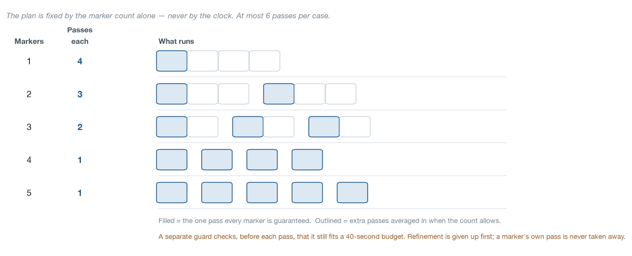
The plan is determined by the number of markers before inference starts. This keeps the amount of computation predictable and avoids making the result depend on how much time happens to remain during execution.
The measured results were:
| Setting | Score |
|---|---|
| No ensemble | 0.7242 |
| Cap 4 | 0.7324 |
| Cap 6 | 0.7361 |
| No cap (4 passes always) | 0.7410 |
The unrestricted ensemble produced the highest score but didn't satisfy the runtime constraint. A cap of 6 retained much of the ensemble improvement while keeping inference within the required limit.
Handle Individual Failures
When processing multiple cases, one failed case shouldn't stop the entire pipeline.
If a case can't be processed, we generate an empty mask and log the error. The pipeline then continues with the remaining cases.
This allows the complete batch to finish even when an individual case has a problem.
The Results
On the 217 hidden test scans, Lumina achieved:
Dice: 0.7619
NSD: 0.6094
The NSD value uses the official 1 mm tolerance.
The median inference time per case was 20.3 seconds. The slowest observed runtime was 31.8 seconds.
Peak memory usage was 2.22 GB inside the 8 GB container.
The Docker image was approximately 559 MB.
Qualitative results
Large lesion with a clear boundary
The first example is a large lesion with a volume of 272.9 cm³. It achieved:
DSC: 0.961
NSD: 0.850
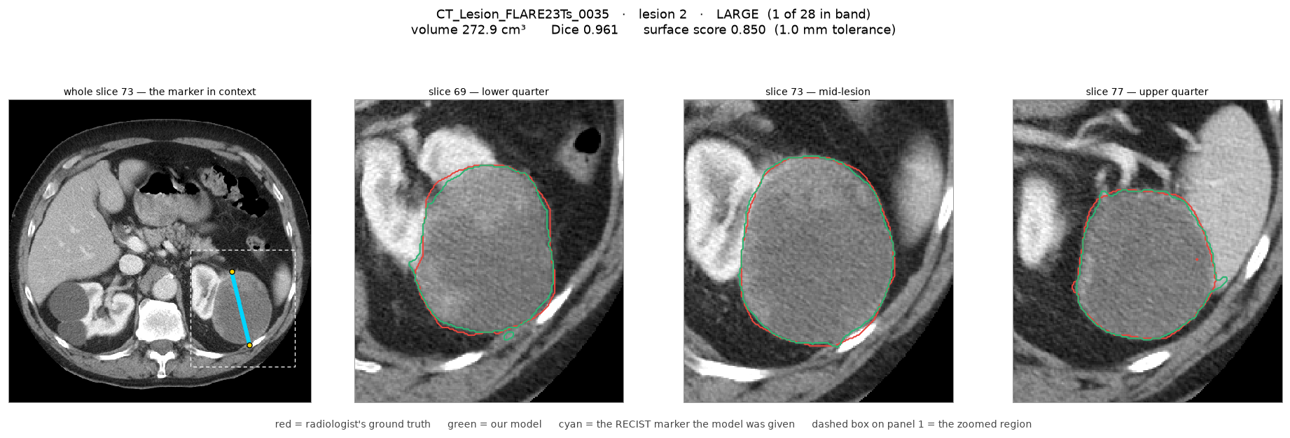
The lesion is well circumscribed, with a clear interface with the surrounding fat.
The predicted contour follows the reference boundary closely across the visible extent of the lesion.
Medium lesion with an uncertain boundary
The second example is a medium lesion with a volume of 28.4 cm³. It achieved:
DSC: 0.563
NSD: 0.114
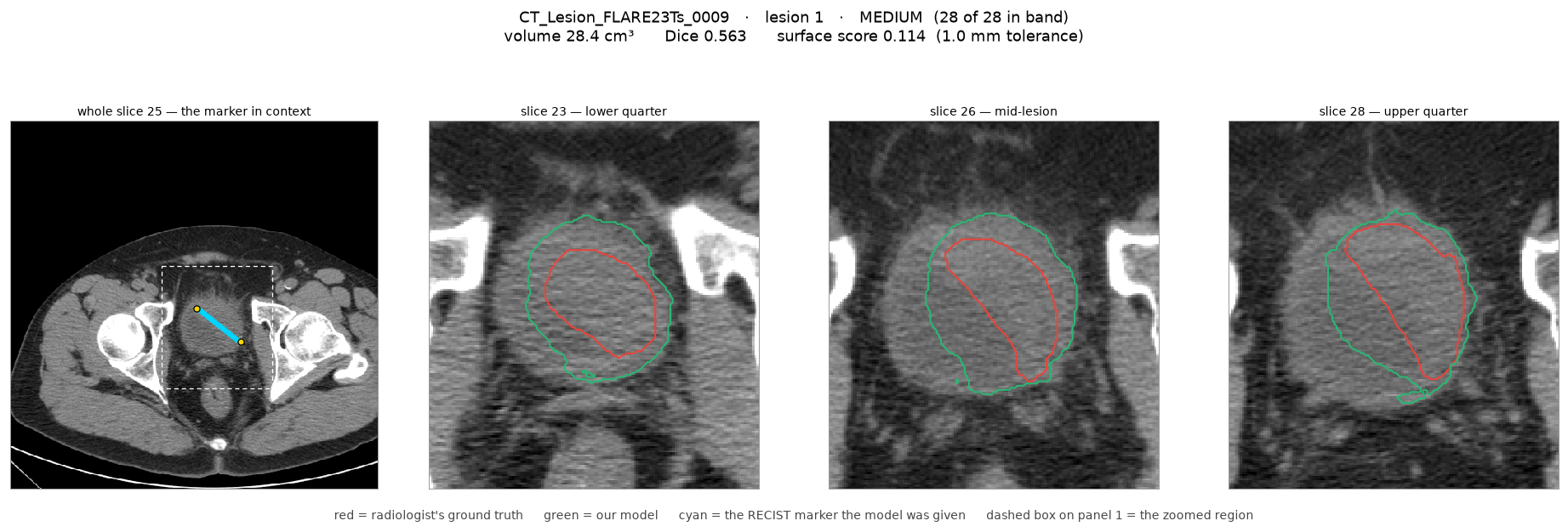
The prediction covers a larger area than the reference annotation.
Radiologist review indicated that this type of case can have uncertainty in the reference boundary itself. Therefore, a low numerical score doesn't by itself establish that the predicted contour is clinically unacceptable.
What the Radiologist Review Showed
We also reviewed 30 lesions with a radiologist to better understand the types of errors Lumina made.
The review showed that lesion size wasn't the only factor affecting segmentation.
Lesions with clear boundaries were generally easier to segment. More difficult cases had poorly defined margins or a similar appearance to the surrounding tissue.
The main errors were:
Under-segmentation: part of the lesion was missed.
Over-segmentation: surrounding tissue was included.
Boundary errors: the predicted contour did not follow an unclear or infiltrative margin.
The review also showed that numerical metrics should be interpreted together with the visible lesion boundary.
In some cases, the reference boundary itself was difficult to define. A low score therefore didn't necessarily mean that the predicted contour was clinically unacceptable.
This is consistent with the lower surface accuracy observed in difficult lesions, where small boundary differences can strongly affect NSD.
Three Lessons That Apply to Other Projects
1. Make Your Validation Data Representative
A validation set should reflect the distribution that the final system will be evaluated on.
Our internal validation split came from the training data. Its median tumor volume was 814 mm³.
The competition scoring set had a median tumor volume of 16,805 mm³, which was much larger.
This difference affected how some improvements appeared during development.
For example, the boundary loss showed little improvement on the internal validation set for several epochs. On the public validation distribution, which contained larger lesions, its effect was more useful.
If an improvement targets a particular part of the data distribution, that distribution should be represented in validation.
2. Measure the Limits of Your Preprocessing
The 160 mm crop was an important design choice in Lumina.
Some large lesions extended beyond this field of view.
Before changing the crop size, we measured the error introduced by cropping and resampling.
We passed the ground-truth masks through the same crop-and-resample pipeline and measured the resulting surface score.
For large lesions, the geometry ceiling was 0.9699 NSD, while the model achieved 0.5353 NSD.
This showed that the preprocessing pipeline preserved the lesion surface reasonably well. Preprocessing alone did not explain the remaining gap.
We also tested several approaches for increasing the field of view, including:
Overlapping tiles
Adaptive zoom
A larger crop
These changes didn't improve the final score.
Measuring the preprocessing ceiling helped us focus further development on the model and inference pipeline.
3. Record Where Your Numbers Come From
Model development involves many configuration values:
Thresholds
Crop sizes
Voxel spacing
Loss weights
Sampling weights
Ensemble settings
Runtime limits
Each value should have a clear source.
For example, record:
What was measured
Which dataset was used
When the measurement was made
Which alternatives were tested
Why the final value was selected.
This makes it easier to reproduce experiments and understand design decisions later.
Conclusion
Lumina shows that a single RECIST line can reconstruct a tumor's 3D extent from a CT scan.
The system combines prompt-based input channels, a fixed physical crop, a 3D DynUNet, boundary-aware training, probability-based post-processing, and controlled CPU inference.
On the 217 held-out cases, Lumina achieved a Dice score of 0.7619 and an NSD of 0.6094 at the official 1 mm tolerance.
The median inference time was 20.3 seconds, with a peak memory usage of 2.22 GB, keeping the system within the challenge constraints.
The experiments also showed that boundary accuracy remains an important area for improvement, particularly for large and less clearly defined lesions.
The geometry-ceiling analysis showed that the crop and resampling pipeline preserved the lesion surface well, indicating that further improvements should focus on segmentation accuracy and robustness.
Overall, Lumina demonstrates a practical approach for converting a 2D RECIST measurement into a 3D lesion segmentation while meeting strict computational constraints.