
By Davis David
When working on a machine learning project, you need to follow a series of steps until you reach your goal.
One of the steps you have to perform is hyperparameter optimization on your selected model. This task always comes after the model selection process where you choose the model that is performing better than other models.
What is hyperparameter optimization?
Before I define hyperparameter optimization, you need to understand what a hyperparameter is.
In short, hyperparameters are different parameter values that are used to control the learning process and have a significant effect on the performance of machine learning models.
An example of hyperparameters in the Random Forest algorithm is the number of estimators (_nestimators), maximum depth (_maxdepth), and criterion. These parameters are tunable and can directly affect how well a model trains.
So then hyperparameter optimization is the process of finding the right combination of hyperparameter values to achieve maximum performance on the data in a reasonable amount of time.
This process plays a vital role in the prediction accuracy of a machine learning algorithm. Therefore Hyperparameter optimization is considered the trickiest part of building machine learning models.
Most of these machine learning algorithms come with the default values of their hyperparameters. But the default values do not always perform well on different types of Machine Learning projects. This is why you need to optimize them in order to get the right combination that will give you the best performance.
A good choice of hyperparameters can really make an algorithm shine.
There are some common strategies for optimizing hyperparameters. Let's look at each in detail now.
How to optimize hyperparameters
Grid Search
This is a widely used and traditional method that performs hyperparameter tuning to determine the optimal values for a given model.
Grid search works by trying every possible combination of parameters you want to try in your model. This means it will take a lot of time to perform the entire search which can get very computationally expensive.
You can learn more about how to implement Grid Search here.
Random Search
This method works a bit differently: random combinations of the values of the hyperparameters are used to find the best solution for the built model.
The drawback of Random Search is that it can sometimes miss important points (values) in the search space.
You can learn more about how to implement Random Search here.
Alternative Hyperparameter Optimization techniques
Now I will introduce you to a few alternative and advanced hyperparameter optimization techniques/methods. These can help you to obtain the best parameters for a given model.
We will look at the following techniques:
- Hyperopt
- Scikit Optimize
- Optuna
Hyperopt
Hyperopt is a powerful Python library for hyperparameter optimization developed by James Bergstra.
It uses a form of Bayesian optimization for parameter tuning that allows you to get the best parameters for a given model. It can optimize a model with hundreds of parameters on a large scale.
Hyperopt has four important features you need to know in order to run your first optimization.
Search Space
Hyperopt has different functions to specify ranges for input parameters. These are called stochastic search spaces. The most common options for a search space are:
- hp.choice(label, options) – This can be used for categorical parameters. It returns one of the options, which should be a list or tuple.
Example:hp.choice("criterion", ["gini","entropy",]) - hp.randint(label, upper) – This can be used for Integer parameters. It returns a random integer in the range (0, upper).
Example:hp.randint("max_features",50) - hp.uniform(label, low, high) – This returns a value uniformly between
lowandhigh.
Example:hp.uniform("max_leaf_nodes",1,10)
Other option you can use are:
- hp.normal(label, mu, sigma) –This returns a real value that's normally distributed with mean mu and standard deviation sigma
- hp.qnormal(label, mu, sigma, q) – This returns a value like round(normal(mu, sigma) / q) * q
- hp.lognormal(label, mu, sigma) – This returns a value drawn according to exp(normal(mu, sigma))
- hp.qlognormal(label, mu, sigma, q) – This returns a value like round(exp(normal(mu, sigma)) / q) * q
You can learn more about search space options here.
Just a quick note: Every optimizable stochastic expression has a label (for example, n_estimators) as the first argument. These labels are used to return parameter choices to the caller during the optimization process.
Objective Function
This is a minimization function that receives hyperparameter values as input from the search space and returns the loss.
This means that during the optimization process, we train the model with selected haypeparameter values and predict the target feature. Then we evaluate the prediction error and give it back to the optimizer.
The optimizer will decide which values to check and iterate again. You will learn how to create objective functions in the practical example.
fmin
The fmin function is the optimization function that iterates on different sets of algorithms and their hyperperameters and then minimizes the objective function.
fmin takes five inputs, which are:
- The objective function to minimize
- The defined search space
- The search algorithm to use, such as Random search, TPE (Tree Parzen Estimators) and Adaptive TPE
Note:hyperopt.rand.suggestandhyperopt.tpe.suggestprovide logic for sequential search of the hyperparameter space - Maximum number of evaluations
- And the trials object (optional)
Example:
from hyperopt import fmin, tpe, hp,Trials

trials = Trials()

best = fmin(fn=lambda x: x ** 2,
            space= hp.uniform('x', -10, 10),
            algo=tpe.suggest,
            max_evals=50,
            trials = trials)

print(best)
Trials Object
The Trials object is used to keep all hyperparameters, loss, and other information. This means you can access it after running the optimization.
Also trials can help you save important information and later load and then resume the optimization process. You will learn more about this in the practical example below.
from hyperopt import Trials

trials = Trials()
Now that you understand the important features of Hyperopt, we'll see how to use it. You'll follow these steps:
- Initialize the space over which to search
- Define the objective function
- Select the search algorithm to use
- Run the hyperopt function
- Analyze the evaluations outputs stored in the trials object
Hyperpot in Practice
In this practical example, we will use the Mobile Price Dataset. Our task is to create a model that will predict how high the price of a mobile device will be: 0 (low cost), 1 (medium cost), 2 (high cost), or 3 (very high cost).
Install Hyperopt
You can install hyperopt from PyPI by running this command:
pip install hyperopt
Then import the following important packages, including hyperopt:
# import packages
import numpy as np
import pandas as pd
from sklearn.ensemble import RandomForestClassifier
from sklearn import metrics
from sklearn.model_selection import cross_val_score
from sklearn.preprocessing import StandardScaler
from hyperopt import tpe, hp, fmin, STATUS_OK,Trials
from hyperopt.pyll.base import scope

import warnings
warnings.filterwarnings("ignore")
Dataset
Let's load the dataset from the data directory. To get more information about the dataset, read about it here.
# load data
data = pd.read_csv("data/mobile_price_data.csv")
Check the first five rows of the dataset like this:
#read data
data.head()
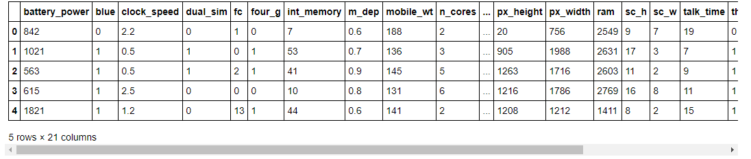 First five rows
As you can see, in our dataset we have different features with numerical values.
Let's look at the shape of the dataset.
#show shape
data.shape
We get the following:
(2000, 21)
In this dataset we have 2000 rows and 21 columns. Now let's understand the list of features we have in this dataset.
#show list of columns
list(data.columns)
['battery_power', 'blue', 'clock_speed', 'dual_sim', 'fc', 'four_g', 'int_memory', 'm_dep', 'mobile_wt', 'n_cores', 'pc', 'px_height', 'px_width', 'ram', 'sc_h', 'sc_w', 'talk_time', 'three_g', 'touch_screen', 'wifi', 'price_range']
You can find the meaning of each column name here .
Splitting the dataset into Target feature and Independent features
This is a classification problem. So we will now split the target feature and independent features from the dataset. Our target feature is price_range.
# split data into features and target
X = data.drop("price_range", axis=1).values
y = data.price_range.values
Preprocessing the Dataset
Next, we'll standardize the independent features by using the StandardScaler method from scikit-learn.
# standardize the feature variables
scaler = StandardScaler()
X_scaled = scaler.fit_transform(X)
Define Parameter Space for Optimization
We will use three hyperparameter of the Random Forest algorithm: _n_estimators, maxdepth, and criterion.
space = {
    "n_estimators": hp.choice("n_estimators", [100, 200, 300, 400,500,600]),
    "max_depth": hp.quniform("max_depth", 1, 15,1),
    "criterion": hp.choice("criterion", ["gini", "entropy"]),
}
We have set different values in the above selected hyperparameters. Now we will define the objective function.
Defining a Function to Minimize (Objective Function)
Our function that we want to minimize is called hyperparamter_tuning. The classification algorithm to optimize its hyperparameter is Random Forest.
I use cross validation to avoid overfitting and then the function will return a loss values and its status.
# define objective function

def hyperparameter_tuning(params):
    clf = RandomForestClassifier(**params,n_jobs=-1)
    acc = cross_val_score(clf, X_scaled, y,scoring="accuracy").mean()
    return {"loss": -acc, "status": STATUS_OK}
Remember that hyperopt minimizes the function. That's why I add the negative sign in the acc.
Fine Tune the Model
Finally, first we'll instantiate the Trial object, fine tune the model, and then print the best loss with its hyperparamters values.
# Initialize trials object
trials = Trials()

best = fmin(
    fn=hyperparameter_tuning,
    space = space,
    algo=tpe.suggest,
    max_evals=100,
    trials=trials
)

print("Best: {}".format(best))
100%|█████████████████████████████████████████████████████████| 100/100 [10:30<00:00, 6.30s/trial, best loss: -0.8915] Best: {'criterion': 1, 'max_depth': 11.0, 'n_estimators': 2}.
After performing hyperparamter optimization, the loss is - 0.8915. This means that the model performance has an accuracy of 89.15% by using _n_estimators = 300, maxdepth = 11, and criterion = "entropy" in the Random Forest classifier.
Analyze the results by using the trials object
The trials object can help us inspect all of the return values that were calculated during the experiment.
(a) trials.results
This show a list of dictionaries returned by 'objective' during the search.
trials.results
[{'loss': -0.8790000000000001, 'status': 'ok'}, {'loss': -0.877, 'status': 'ok'}, {'loss': -0.768, 'status': 'ok'}, {'loss': -0.8205, 'status': 'ok'}, {'loss': -0.8720000000000001, 'status': 'ok'}, {'loss': -0.883, 'status': 'ok'}, {'loss': -0.8554999999999999, 'status': 'ok'}, {'loss': -0.8789999999999999, 'status': 'ok'}, {'loss': -0.595, 'status': 'ok'},.......]
(b) trials.losses()
This shows a list of losses (float for each 'ok' trial).
trials.losses()
[-0.8790000000000001, -0.877, -0.768, -0.8205, -0.8720000000000001, -0.883, -0.8554999999999999, -0.8789999999999999, -0.595, -0.8765000000000001, -0.877, .........]
(c) trials.statuses()
This shows a list of status strings.
trials.statuses()
['ok', 'ok', 'ok', 'ok', 'ok', 'ok', 'ok', 'ok', 'ok', 'ok', 'ok', 'ok', 'ok', 'ok', 'ok', 'ok', 'ok', 'ok', 'ok', ..........]
Note: This trials object can be saved, passed on to the built-in plotting routines, or analyzed with your own custom code.
Now that you know how to implement Hyperopt, let's learn the second alternative hyperparameter optimization technique called Scikit-Optimize.
Scikit-Optimize
Scikit-optimize is another open-source Python library for hyperparameter optimization. It implements several methods for sequential model-based optimization.
The library is very easy to use and provides a general toolkit for Bayesian optimization that can be used for hyperparameter tuning. It also provides support for tuning the hyperparameters of machine learning algorithms offered by the scikit-learn library.
The scikit-optimize is built on top of Scipy, NumPy, and Scikit-Learn.
Scikit-optimize has at least four important features you need to know in order to run your first optimization. Let's look at them in depth now.
Space
scikit-optimize has different functions to define the optimization space which contains one or multiple dimensions. The most common options for a search space to choose are:
- Real — This is a search space dimension that can take on any real value. You need to define the lower bound and upper bound and both are inclusive.
Example:Real(low=0.2, high=0.9, name="min_samples_leaf") - Integer — This is a search space dimension that can take on integer values.
Example:Integer(low=3, high=25, name="max_features") - Categorical — This is a search space dimension that can take on categorical values.
Example:Categorical(["gini","entropy"],name="criterion")
Note: in each search space you have to define the hyperparameter name to optimize by using the name argument.
BayesSearchCV
The BayesSearchCV class provides an interface similar to GridSearchCV or RandomizedSearchCV but it performs Bayesian optimization over hyperparameters.
BayesSearchCV implements a “fit” and a “score” method and other common methods like _predict(),predict_proba(), decisionfunction(), transform() and _inversetransform() if they are implemented in the estimator used.
In contrast to GridSearchCV, not all parameter values are tried out. Rather a fixed number of parameter settings is sampled from the specified distributions. The number of parameter settings that are tried is given by n_iter.
Note that you will learn how to implement BayesSearchCV in a practical example below.
Objective Function
This is a function that will be called by the search procedure. It receives hyperparameter values as input from the search space and returns the loss (the lower the better).
This means that during the optimization process, we train the model with selected hyperparameter values and predict the target feature. Then we evaluate the prediction error and give it back to the optimizer.
The optimizer will decide which values to check and iterate over again. You will learn how to create an objective function in the practical example below.
Optimizer
This is the function that performs the Bayesian Hyperparameter Optimization process. The optimization function iterates at each model and the search space to optimize and then minimizes the objective function.
There are different optimization functions provided by the scikit-optimize library, such as:
- dummy_minimize — Random search by uniform sampling within the given bounds.
- forest_minimize — Sequential optimization using decision trees.
- gbrt_minimize — Sequential optimization using gradient boosted trees.
- gp_minimize — Bayesian optimization using Gaussian Processes.
Note: we will implement gp_minimize in the practical example below.
Other features you should learn are as follow:
- Space Transformers
- Utils Functions
- Plotting Functions
- Machine learning extensions for model-based optimization
Scikit-optimize in Practice
Now that you know the important features of scikit-optimize, let's look at a practical example. We will use the same dataset called Mobile Price Dataset that we used with Hyperopt.
Install Scikit-Optimize
scikit-optimize requires the following Python version and packages:
- Python >= 3.6
- NumPy (>= 1.13.3)
- SciPy (>= 0.19.1)
- joblib (>= 0.11)
- scikit-learn >= 0.20
- matplotlib >= 2.0.0
You can install the latest release with this command:
pip install scikit-optimize
Then import important packages, including scikit-optimize:
# import packages
import numpy as np
import pandas as pd
from sklearn.ensemble import RandomForestClassifier
from sklearn import metrics
from sklearn.model_selection import cross_val_score
from sklearn.preprocessing import StandardScaler
from skopt.searchcv import BayesSearchCV
from skopt.space import Integer, Real, Categorical
from skopt.utils import use_named_args
from skopt import gp_minimize

import warnings

warnings.filterwarnings("ignore")
The First Approach
In the first approach, we will use BayesSearchCV to perform hyperparameter optimization for the Random Forest algorithm.
Define Search Space
We will tune the following hyperparameters of the Random Forest model:
- n_estimators — The number of trees in the forest.
- max_depth — The maximum depth of the tree.
- criterion — The function to measure the quality of a split.
# define search space
params = {
    "n_estimators": [100, 200, 300, 400],
    "max_depth": (1, 9),
    "criterion": ["gini", "entropy"],
}
We have defined the search space as a dictionary. It has hyperparameter names used as the key, and the scope of the variable as the value.
Define the BayesSearchCV configuration
The benefit of BayesSearchCV is that the search procedure is performed automatically, which requires minimal configuration.
The class can be used in the same way as Scikit-Learn (GridSearchCV and RandomizedSearchCV).
# define the search
search = BayesSearchCV(
    estimator=rf_classifier,
    search_spaces=params,
    n_jobs=1,
    cv=5,
    n_iter=30,
    scoring="accuracy",
    verbose=4,
    random_state=42
)
Fine Tune the Model
We then execute the search by passing the preprocessed features and the target feature (price_range).
# perform the search
search.fit(X_scaled,y)
You can find the best score by using the bestscore attribute and the best parameters by using bestparams attribute from the search.
# report the best result

print(search.best_score_)
print(search.best_params_)
Note that the current version of scikit-optimize (0.7.4) is not compatible with the latest versions of scikit learn (0.23.1 and 0.23.2). So when you run the optimization process using this approach, you can get errors like this:
TypeError: object.__init__() takes exactly one argument (the instance to initialize)
You can find more information about this error in their GitHub account.
- https://github.com/scikit-optimize/scikit-optimize/issues/928
- https://github.com/scikit-optimize/scikit-optimize/issues/924
- https://github.com/scikit-optimize/scikit-optimize/issues/902
I hope they will solve this incompatibility problem very soon.
The Second Approach
In the second approach, we first define the search space by using the space methods provided by scikit-optimize, which are Categorical and Integer.
# define the space of hyperparameters to search
search_space = list()
search_space.append(Categorical([100, 200, 300, 400], name='n_estimators'))
search_space.append(Categorical(['gini', 'entropy'], name='criterion'))
search_space.append(Integer(1, 9, name='max_depth'))
We have set different values in the above-selected hyperparameters. Then we will define the objective function.
Defining a Function to Minimize (Objective Function)
Our function to minimize is called evalute_model and the classification algorithm to optimize its hyperparameter is Random Forest.
I use cross-validation to avoid overfitting and then the function will return loss values.
# define the function used to evaluate a given configuration

@use_named_args(search_space)
def evaluate_model(**params):
    # configure the model with specific hyperparameters
    clf = RandomForestClassifier(**params, n_jobs=-1)
    acc = cross_val_score(clf, X_scaled, y, scoring="accuracy").mean()
The use_named_args() decorator allows your objective function to receive the parameters as keyword arguments. This is particularly convenient when you want to set scikit-learn's estimator parameters.
Remember that scikit-optimize minimizes the function, which is why I add a negative sign in the acc.
Fine Tune the Model
Finally, we fine-tune the model by using the gp_minimize method (it uses Gaussian process-based optimization) from scikit-optimize. Then we print the best loss with its hyperparameters values.
# perform optimization

result = gp_minimize(
    func=evaluate_model,
    dimensions=search_space,
    n_calls=30,
    random_state=42,
    verbose=True,
    n_jobs=1,
)
Output:
Iteration No: 1 started. Evaluating function at random point.
Iteration No: 1 ended. Evaluation done at random point.
Time taken: 8.6910
Function value obtained: -0.8585
Current minimum: -0.8585
Iteration No: 2 started. Evaluating function at random point.
Iteration No: 2 ended. Evaluation done at random point.
Time taken: 4.5096
Function value obtained: -0.7680
Current minimum: -0.8585 ………………….
Not that it will run until it reaches the last iteration. For our optimization process, the total number of iterations is 30.
Then we can print the best accuracy and the values of the selected hyperparameters we used.
# summarizing finding:

print('Best Accuracy: %.3f' % (result.fun))
print('Best Parameters: %s' % (result.x))
Best Accuracy: -0.882
Best Parameters: [300, 'entropy', 9]
After performing hyperparameter optimization, the loss is -0.882. This means that the model's performance has an accuracy of 88.2% by using _nestimators = 300, _maxdepth = 9, and criterion = “entropy” in the Random Forest classifier.
Our result is not much different from Hyperopt in the first part (accuracy of 89.15%).
Print Function Values
You can print all function values at each iteration by using the func_vals attribute from the OptimizeResult object (result).
print(result.func_vals)
Output:
array([-0.8665, -0.7765, -0.7485, -0.86 , -0.872 , -0.545 , -0.81 ,
-0.7725, -0.8115, -0.8705, -0.8685, -0.879 , -0.816 , -0.8815,
-0.8645, -0.8745, -0.867 , -0.8785, -0.878 , -0.878 , -0.8785,
-0.874 , -0.875 , -0.8785, -0.868 , -0.8815, -0.877 , -0.879 ,
-0.8705, -0.8745])
Plot Convergence Traces
We can use the plot_convergence method from scikit-optimize to plot one or several convergence traces. We just need to pass the OptimizeResult object (result) in the plot_convergence method.
# plot convergence

from skopt.plots import plot_convergence

plot_convergence(result)

The plot shows function values at different iterations during the optimization process.
Now that you know how to implement scikit-optimize, let's learn the third and final alternative hyperparameter optimization technique called Optuna.
Optuna
Optuna is another open-source Python framework for hyperparameter optimization that uses the Bayesian method to automate search space of hyperparameters. The framework was developed by a Japanese AI company called Preferred Networks.
Optuna is easier to implement and use than Hyperopt. You can also specify how long the optimization process should last.
Optuna has at least five important features you need to know in order to run your first optimization.
Search Spaces
Optuna provides different options for all hyperparameter types. The most common options to choose are as follows:
- Categorical parameters – uses the trials.suggest_categorical() method. You need to provide the name of the parameter and its choices.
- Integer parameters – uses the trials.suggest_int() method. You need to provide the name of the parameter, low and high value.
- Float parameters – uses the trials.suggest_float() method. You need to provide the name of the parameter, low and high value.
- Continuous parameters – uses the trials.suggest_uniform() method. You need to provide the name of the parameter, low and high value.
- Discrete parameters – uses the trials.suggest_discrete_uniform() method. You need to provide the name of the parameter, low value, high value, and step of discretization.
Optimization methods (Samplers)
Optuna has different ways to perform the hyperparameter optimization process. The most common methods are:
- GridSampler – It uses a grid search. The trials suggest all combinations of parameters in the given search space during the study.
- RandomSampler – It uses random sampling. This sampler is based on independent sampling.
- TPESampler – It uses the TPE (Tree-structured Parzen Estimator) algorithm.
- CmaEsSampler – It uses the CMA-ES algorithm.
Objective Function
The objective function works the same way as in the hyperopt and scikit-optimize techniques. The only difference is that Optuna allows you to define the search space and objective in the one function.
Example:
def objective(trial):
    # Define the search space
    criterions = trial.suggest_categorical('criterion', ['gini', 'entropy'])
    max_depths = trial.suggest_int('max_depth', 1, 9, 1)
    n_estimators = trial.suggest_int('n_estimators', 100, 1000, 100)

    clf = sklearn.ensemble.RandomForestClassifier(n_estimators=n_estimators,
                                 criterion=criterions,
                                 max_depth=max_depths,
                                 n_jobs=-1)

    score = cross_val_score(clf, X_scaled, y, scoring="accuracy").mean()

    return score
(d) Study
A study corresponds to an optimization task (a set of trials). If you need to start the optimization process, you need to create a study object and pass the objective function to a method called optimize() and set the number of trials as follows:
study = optuna.create_study()
study.optimize(objective, n_trials=100)
The create_study() method allows you to choose whether you want to maximize or minimize your objective function.
This is one of the more useful features I like in optuna because you have the ability to choose the direction of the optimization process.
Note that you will learn how to implement this in the practical example below.
Visualization
The visualization module in Optuna provides different methods to create figures for the optimization outcome. These methods help you gain information about interactions between parameters and let you know how to move forward.
Here are some of the methods you can use.
- plot_contour() – This method plots the parameter relationship as a contour plot in a study.
- plot_intermidiate_values() – This method plots intermediate values of all trials in a study.
- plot_optimization_history() – This method plots the optimization history of all trials in a study.
- plot_param_importances() – This method plots hyperparameter importance and their values.
- plot_edf() – This method plots the objective value EDF (empirical distribution function) of a study.
We will use some of the methods mentioned above in the practical example below.
Optuna in Practice
Now that you know the important features of Optuna, in this practical example we will use the same dataset (Mobile Price Dataset) that we used in the previous two methods above.
Install Optuna
You can install the latest release with:
pip install optuna
Then import the important packages, including optuna:
# import packages
import numpy as np
import pandas as pd
from sklearn.ensemble import RandomForestClassifier
from sklearn import metrics
from sklearn.model_selection import cross_val_score
from sklearn.preprocessing import StandardScaler
import joblib

import optuna
from optuna.samplers import TPESampler


import warnings
warnings.filterwarnings("ignore")
Define search space and objective in one function
As I have explained above, Optuna allows you to define the search space and objective in one function.
We will define the search spaces for the following hyperparameters of the Random Forest model:
- n_estimators — The number of trees in the forest.
- max_depth — The maximum depth of the tree.
- criterion — The function to measure the quality of a split.
# define the search space and the objecive function


def objective(trial):
    # Define the search space
    criterions = trial.suggest_categorical('criterion', ['gini', 'entropy'])
    max_depths = trial.suggest_int('max_depth', 1, 9, 1)
    n_estimators = trial.suggest_int('n_estimators', 100, 1000, 100)

    clf = RandomForestClassifier(n_estimators=n_estimators,
                                 criterion=criterions,
                                 max_depth=max_depths,
                                 n_jobs=-1)
    score = cross_val_score(clf, X_scaled, y, scoring="accuracy").mean()

    return score
We will use the trial.suggest_categorical() method to define a search space for criterion and trial.suggest_int() for both _maxdepth and _nestimators.
Also, we will use cross-validation to avoid overfitting, and then the function will return the mean accuracy.
Create a Study Object
Next we create a study object that corresponds to the optimization task. The create-study() method allows us to provide the name of the study, the direction of the optimization (maximize or minimize), and the optimization method we want to use.
# create a study object

study = optuna.create_study(study_name="randomForest_optimization",
                            direction="maximize",
                            sampler=TPESampler())
In our case we named our study object randomForest_optimization. The direction of the optimization is maximize (which means the higher the score the better) and the optimization method to use is TPESampler().
Fine Tune the Model
To run the optimization process, we need to pass the objective function and number of trials in the optimize() method from the study object we have created.
We have set the number of trials to be 10 (but you can change the number if you want to run more trials).
# pass the objective function to method optimize()

study.optimize(objective, n_trials=10)
Output:**
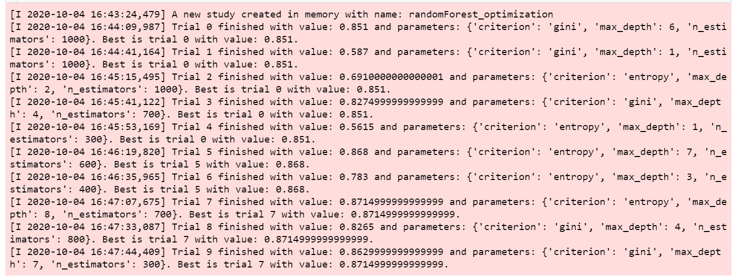
Then we can print the best accuracy and the values of the selected hyperparameters used.
To show the best hyperparameters values selected:
print(study.best_params)
Output: {‘criterion’: ‘entropy’, ‘max_depth’: 8, ‘n_estimators’: 700}
To show the best score or accuracy:
print(study.best_value)
Output: 0.8714999999999999.
Our best score is around 87.15%.
Plot Optimization History
We can use the plot_optimization_history() method from Optuna to plot the optimization history of all trials in a study. We just need to pass the optimized study object in the method.
optuna.visualization.plot_optimization_history(study)
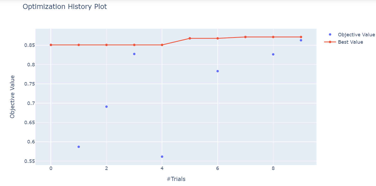
The plot shows the best values at different trials during the optimization process.
Plot Hyperparameter Importances
Optuna provides a method called plot_param_importances() to plot hyperparameter importance. We just need to pass the optimized study object in the method.
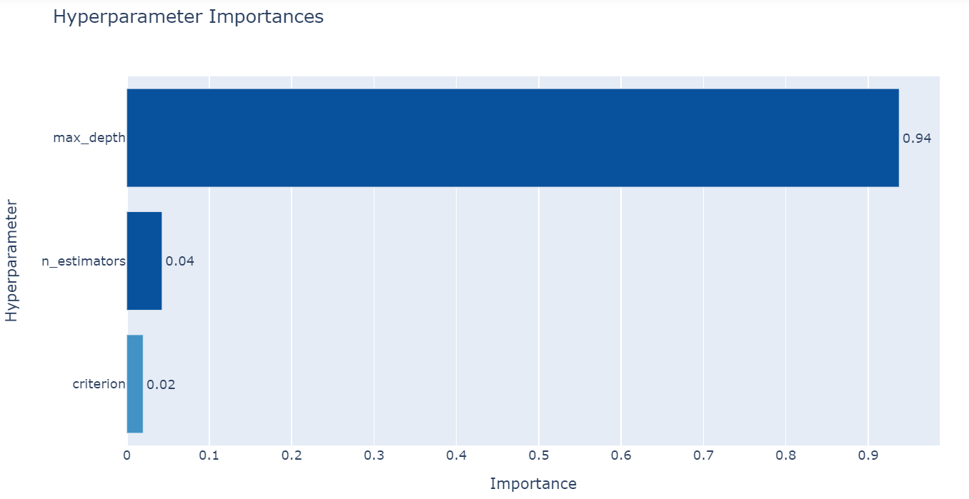
From the figure above you can see that max-depth is the most important hyperparameter.
Save and Load Hyperparameter Searches
You can save and load the hyperparameter searches by using the joblib package.
First, we will save the hyperparameter searches in the optuna_searches directory.
# save your hyperparameter searches

joblib.dump(study, 'optuna_searches/study.pkl')
Then if you want to load the hyperparameter searches from the optuna_searches directory, you can use the load() method from joblib.
# load your hyperparameter searches

study = joblib.load('optuna_searches/study.pkl')
Wrapping Up
Congratulations, you have made it to the end of the article!
Let’s take a look at the overall scores and hyperparameter values selected by the three hyperparameter optimization techniques we have discussed in this article.
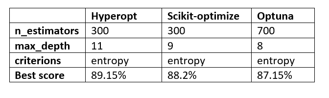
The results presented by each technique are not that different from each other. The number of iterations or trials selected makes all the difference.
For me, Optuna is easy to implement and is my first choice in hyperparameter optimization techniques. Please let me know what you think!
You can download the dataset and all notebooks used in this article here:
https://github.com/Davisy/Hyperparameter-Optimization-Techniques
If you learned something new or enjoyed reading this article, please share it so that others can see it. Until then, see you in my next article!. I can also be reached on Twitter @Davis_McDavid