

Machine learning models are black box models. By giving input to these models, we can get output based on the particular model we're using.
The way humans interpret things is different from how machines interpret them. So it's helpful to use tools that can turn the output from certain machine learning models into something humans or non-technical users can understand.
In a business context, the interpretation of the model plays an important role in making data-driven decisions. The better we interpret the output, the easier it is for non-technical users to understand that output.
So in this tutorial, I will explain one of most popular packages you can use for interpreting the black box model of the output – a package called LIME (Local Interpretable Model-Agnostic Explanations).
What is LIME?
LIME is a model-agnostic machine learning tool that helps you interpret your ML models. The term model-agnostic means that you can use LIME with any machine learning model when training your data and interpreting the results.
LIME uses "inherently interpretable models" such as decision trees, linear models, and rule-based heuristic models to explain results to non-technical users with visual forms. You can use LIME for regression and classification problems to interpret your black box models.
Gathering the Data
In this tutorial, we will look at a classification problem using the Churn dataset. We will classify whether customers will keep using products or not (churn rate) by looking at some features in the dataset.
You can download the Kaggle telco customers churn dataset here.
Data Preprocessing
Because this tutorial is focussing on the implementation of LIME as an interpretability tool, we will just do a few preprocessing steps for various features.
We start preprocessing by going over the columns that aren't relevant to the target outcome (churn). You can delete the CustomerID by using this code:
# Dropping all irrelevant columns
df.drop(columns=['customerID'], inplace = True)
We also have a few missing values that aren't properly imputing. For simplicity's sake, we just deleted the missing values by using this code:
# Dropping missing values
df.dropna(inplace=True)
Another preprocessing step that we should do is to look at the categorical columns. The vast majority of machine learning models can not handle categorical features. So we have to preprocess this type of feature into a numerical representation.
There are various transformations that we can do such as label encoding, hashing tricks, one hot encoding, target encoding, Ordinal encoding, and frequency encoding.
For this tutorial, we're going to use the label encoding technique using the scikit-learn library as shown in the following code:
# Label Encoding features
categorical_feat =list(df.select_dtypes(include=["object"]))

# Using label encoder to transform string categories to integer labels
le = LabelEncoder()
for feat in categorical_feat:
    df[feat] = le.fit_transform(df[feat]).astype('int')
It is worth noting that when you're working on an actual ML problem/dataset, you'll want to make sure you carry out proper preprocessing, feature engineering, cross validation, hyperparameter tuning, and so on to get a better prediction.
Modeling with XGBoostClassifier and LIME implementation
XGBoostClassifier is an XGBoost algorithm that you can use for solving classification problems. It works by constructing the data into a decision tree and using the residuals to be constructed again into the next decision tree sequentially.
This algorithm helps you improve the performance of your model's predictions that can resemble the ground truth. This is because it improves misclassified predictions (weak learners) by helping them become strong learners. It does this through learning the misclassified prediction that is used upon the next iteration of next decision tree.
You can check out the following diagram to see how this algorithm works:
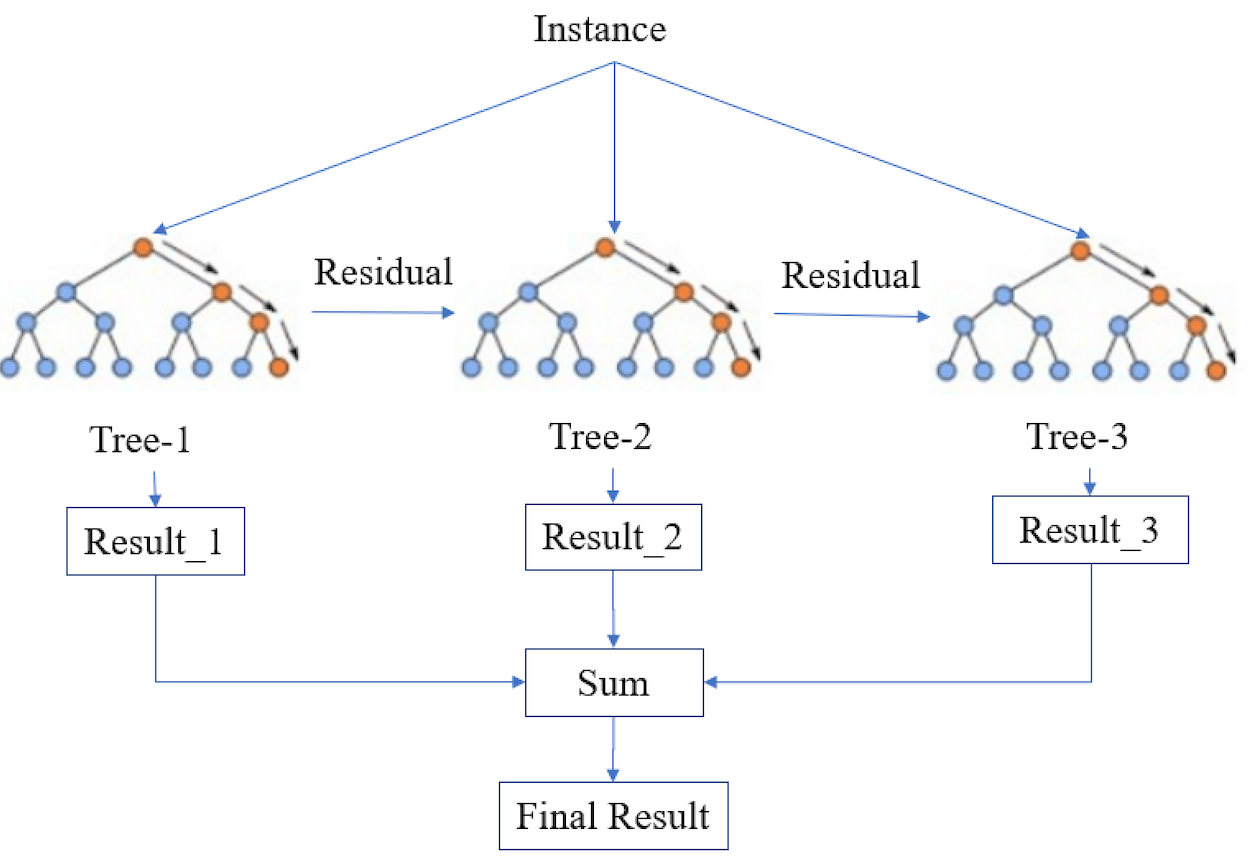 _Figure 4. Simplified XGBoost (source)_
We can implement LIME after going through the training process on our training data.
We start the training process by splitting the data into training and test datasets in order to avoid overfitting. We can use the splitting method available in scikit-learn as shown in the following code:
features = df.drop(columns=['Churn'])
labels = df['Churn']
# Dividing the data into training-test set with 80:20 split ratio
x_train,x_test,y_train,y_test = train_test_split(features,labels,test_size=0.2, random_state=123)
We select the features and the target outcome (churn) and split the data into train and test data. Then, we can start training by fitting the X_train and y_train based on the instantiating object of the machine learning model that we're using. We're using XGBoostClassifier for this tutorial.
We initialize n_estimators (number of decision trees) and random state for the simplicity of the training process. In a real data science project, there are many parameters that you'll want to tweak in order to maximize the capability of this algorithm. You can refer to XGBoost parameters to learn more.
model = XGBClassifier(n_estimators = 300, random_state = 123)
model.fit(x_train, y_train)
After fitting the data through the training process, we will work on interpreting local interpretability. Local Interpretability involves analyzing each feature of a particular data instance. We can select a particular instance/sample to check how the features correlate to the target outcome based on a particular sample.
np.random.seed(123)
predict_fn = lambda x: model.predict_proba(x)
# Defining the LIME explainer object
explainer = lime.lime_tabular.LimeTabularExplainer(df[features.columns].astype(int).values,                                               mode='classification',
class_names=['Did not Churn', 'Churn'],                                                 training_labels=df['Churn'],                                                  feature_names=features.columns)
# using LIME to get the explanations
i = 5
exp=explainer.explain_instance(df.loc[i,features.columns].astype(int).values, predict_fn, num_features=5)
exp.show_in_notebook(show_table=True)
To get the explanation for a particular instance, we start by defining a function as the probability score that will be utilized on the LIME framework. We also instantiate the LIME explainer object.
LIME has an attribute lime_tabular that can interpret how the features correlate to the target outcome. We can also specify the mode to classification, training_label to the target outcome (Churn), and the features that we have selected on the training process.
We choose sample 5 and we'll get the explanation for this particular sample. We also choose the 5 most important features that contribute the most to the target outcome on the num_features parameter.
These features are also called feature importance. Feature Importance is the feature that checks the correlation between the input features and the target features. The higher the score of the feature in the feature importance plot, the more important the feature is to be fitted into the machine learning model.
How to Interpret Local Interpretability
 Figure 8. Local Interpretability Prediction
The above image shows three graphs that each show essential information about our customers and their churn rates.
The left graph shows that sample 5 in the data shows the confidence interval stating that this data is 99% churn whereas only 1% indicates the instance did not churn.
The center graph shows the feature importance scores on this particular sample with MonthlyCharges having a 21% feature importance score, followed by Contract with 19% and tenure with 11%. These features make sense based on our belief that customers tend to churn more on the higher MonthlyCharge.
The right graph shows the top five features and their respective values. The features highlighted in orange contribute toward class 1 (Churn) whereas features highlighted in blue contribute toward class 0 (not Churn).
We can also plot another version of the second graph as shown in the following bar plot. It shows the range of local interpretability predictions on sample 5 in which MonthlyCharges for this particular sample are greater than 89, Contract is less than 0, and totalCharges is greater than 401 and less than 1397.
 Figure 9. The range of Local Interpretability Prediction
How to Interpret Global Interpretability
LIME also provides another explanation through the SP-LIME algorithm that takes representative samples to extract the global perspective from the black box model.
This technique helps non-technical users understand the data not only in a particular instance (local interpretability) but also it also helps them understand the data holistically. By understanding many representative samples and their interpretations, non-technical users can capture the global perspective of the data instances.
# Let's use SP-LIME to return explanations on a few sample data sets
# and obtain a non-redundant global decision perspective of the black-box model
sp_exp = submodular_pick.SubmodularPick(explainer,
                                        df[features.columns].values,
                                        predict_fn,
                                        num_features=5,
                                        num_exps_desired=5)
We use the sub-modular attributes available on SP-LIME to obtain a global perspective of the data instances. Then, we visualize the data to visual global representative samples extracted by the SP-LIME algorithm using this code:
[exp.show_in_notebook() for exp in sp_exp.sp_explanations]
print('SP-LIME Explanations.')
 Figure 12. The range of global interpretability Prediction
You can see how SP-LIME constructs interval values for each representative sample. For instance, the first representative sample shows the confidence interval is 81% Churn whereas 19% indicates that the instances do not churn.
The features that influence how this instance tends to churn are MonthlyCharge, Contract, tenure,OnlineSecurity, and TechSupport. You can see this in the below feature importance bar plot for the first representative sample. We can also plot another version of the middle plot of each representative sample on the preceding graph using this code:
[exp.as_pyplot_figure(label=exp.available_labels()[0]) for exp in sp_exp.sp_explanations]
print('SP-LIME Local Explanations')
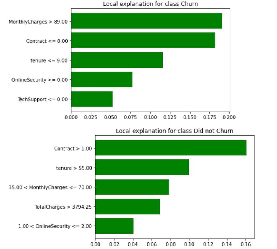 Figure 14. First and Second Representative samples
On the second representative sample on figure 12, the confidence interval is 100% not Churn. The features that influence how this instance tends to not churn are Contract, tenure, MonthlyCharge, TotalCharges, and OnlineSecurity as shown on the following feature importance bar plot for the second representative sample.
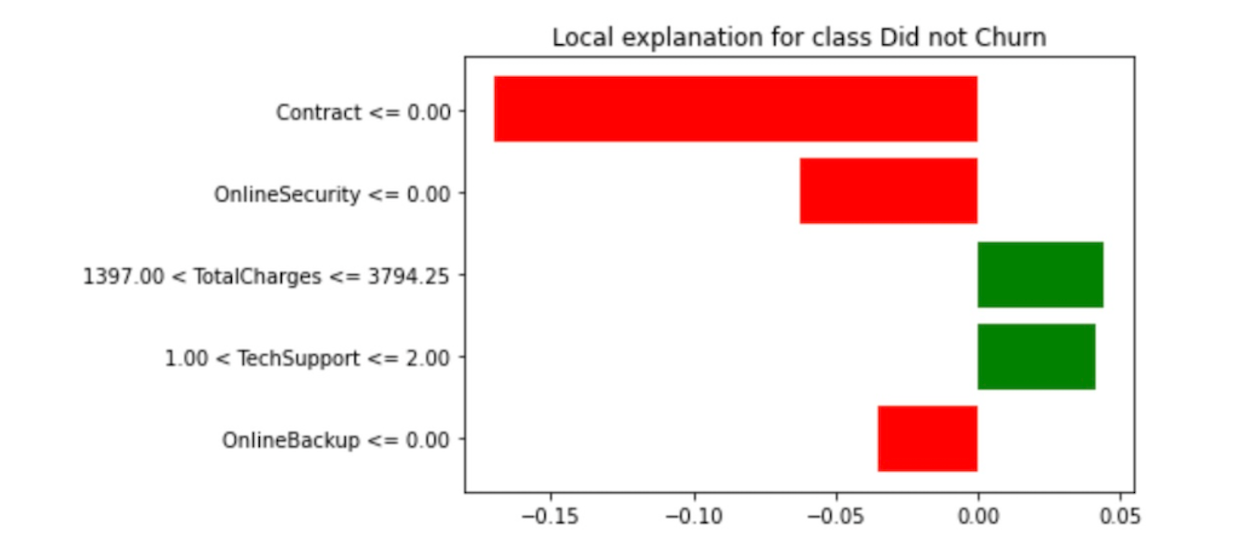 Figure 15. Third representative sample
On the third representative sample on figure 12, the confidence interval is 100% not Churn. The features that influence how this instance tends to not churn are Contract, OnlineSecurity, and OnlineBackup as shown on the above feature importance plot for the third representative sample.
You can see the implementation of LIME and SP-LIME on the data by looking at this notebook.
Here's an interesting article about trusting models.
Thank you for reading!
I really appreciate it! 🤗 . I write about topics related to machine learning and deep learning. I try to keep my posts simple but precise, always providing visualizations and simulations.