
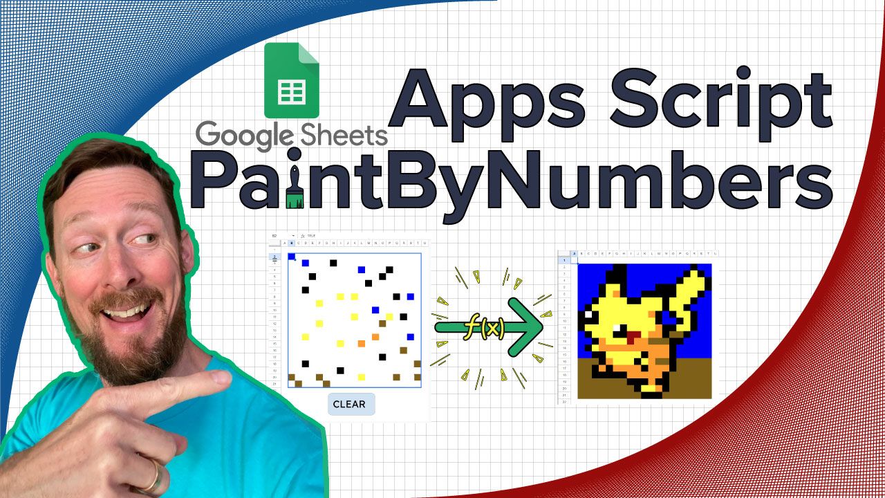
Spreadsheets are great for financial modeling, but they're also capable of displaying pixel art.
In this Apps Script tutorial, we'll build a paint by numbers spreadsheet using conditional formatting and a script that "paints" a blank spreadsheet.
You'll learn how to:
- Import data
- Apply proper data visualization formatting to it
- Code a couple of Apps Script functions to make it interactive.
Let's do it 🎨
 Tenacious D rocking out
Video Walkthrough
Yes, I've got a full walkthrough for you. Pull this up as you read to reference and follow along 👇
Demo sheet with Pikachu: https://docs.google.com/spreadsheets/d/1Zu0B0dE_N4UrgAAzlWKqbpmz2TL_qr9GYWS451O7UL0/edit#gid=0
Demo sheet with Volcano: https://docs.google.com/spreadsheets/d/11lOVseXtpB6xWxhrmZr1LfImI75TBDbof6mkFzz0ck4/edit#gid=0
You can make an editable copy of either of these by selecting File -> Make a copy.
Project Setup
Everything we're doing today is built on some simple formatting. We are going to have cells turn certain colors based on the number inside them.
See the pic below where all the blue cells have the number 15 in them. By setting the color of the font and the background to blue, we can create the effect of the cells being a solid color.
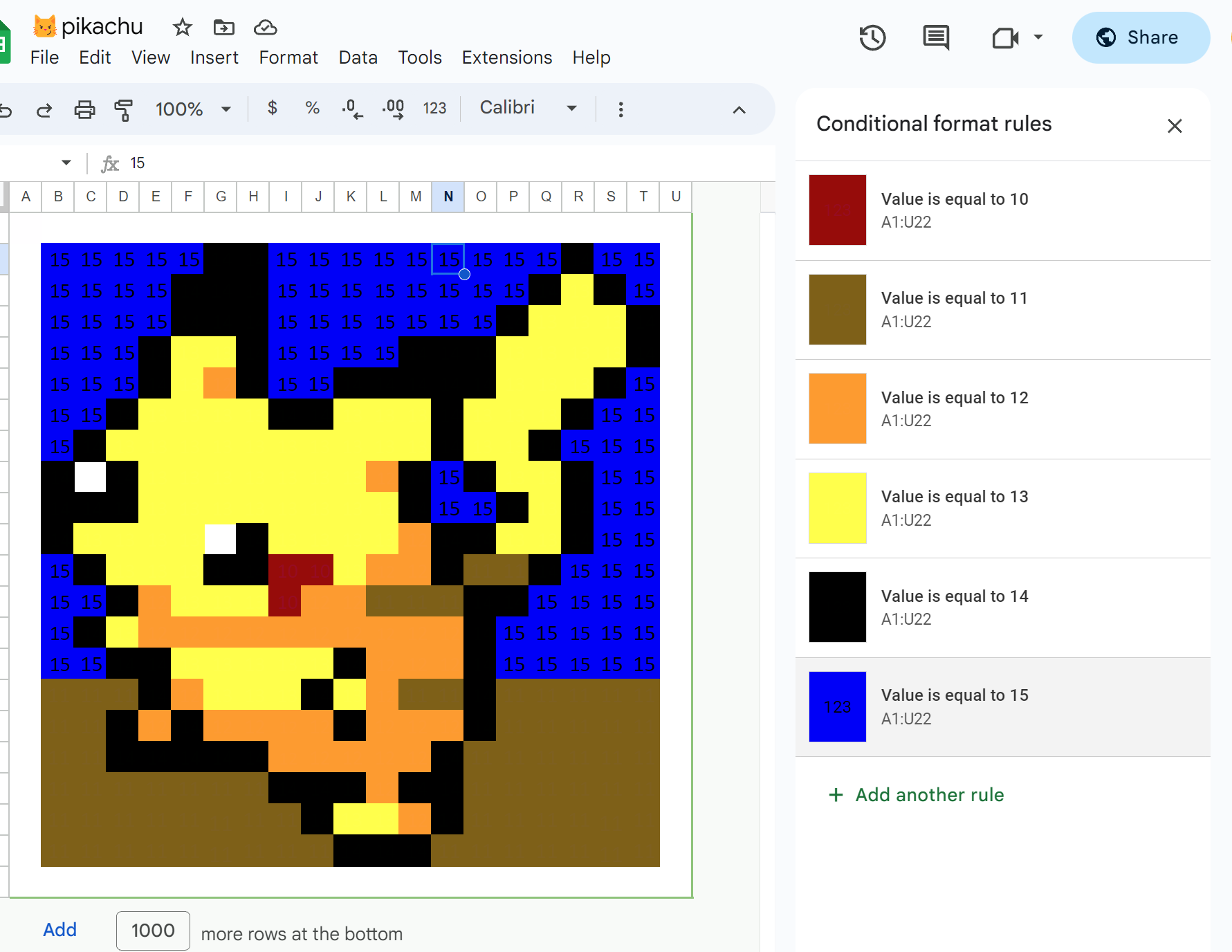 Picture of Pikachu pixel artwork
We can make our own number grid, but there are a ton available. I print these for my kids to color, and we can import them to our spreadsheet with a couple clicks.
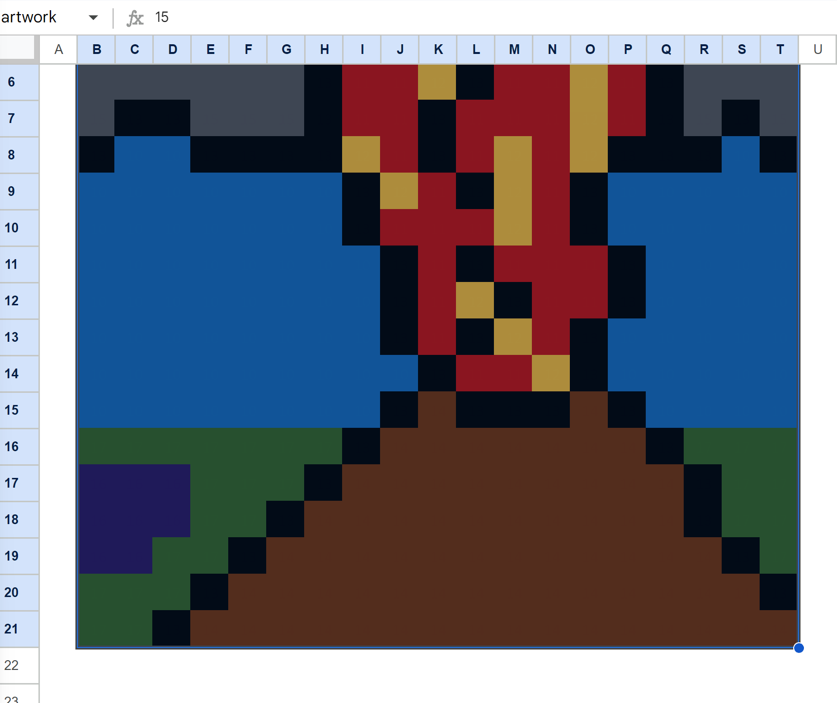
Here's the volcano grid I used in the walkthrough video.
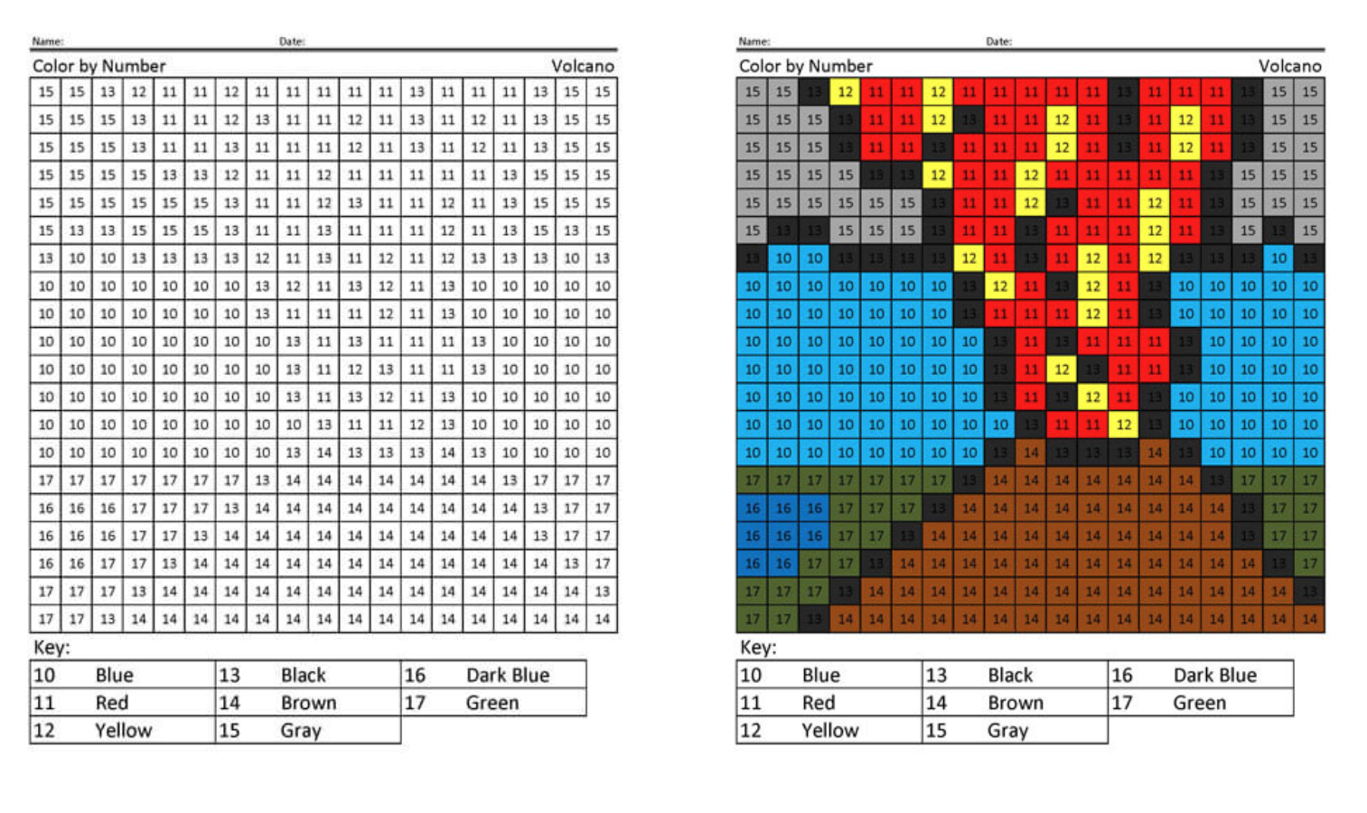 Picture of volcano color by number grid
When I first recorded the walkthrough video, I was unable to copy and paste from the PDF. When I did, it pasted every number in one cell.
Instead, by opening in Microsoft Word first and then copying and pasting from there, I was able to bring the number grid into the Google Sheet.
Since then, I've also found that when copying and pasting from the PDF, sometimes it will bring the numbers in to the first cell in each row:
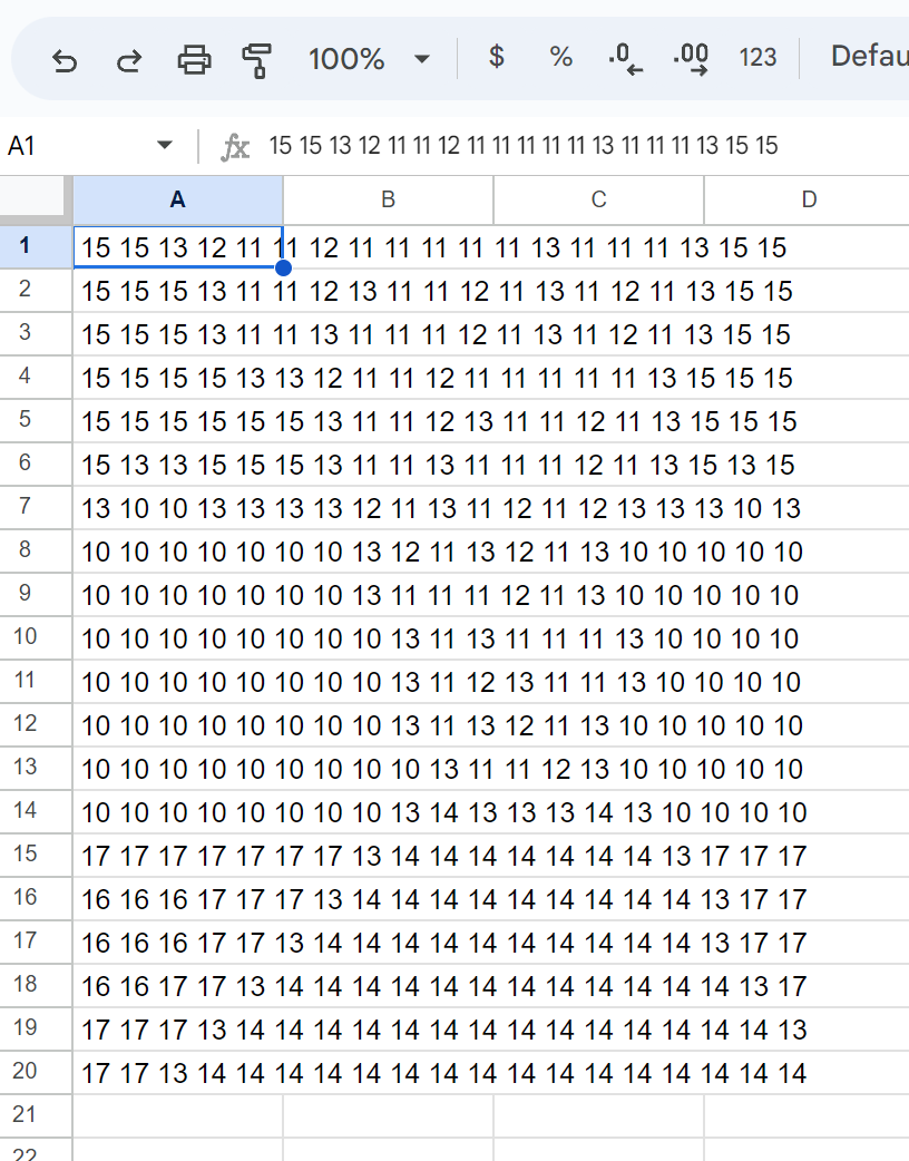 picture of Google Sheets number grid
This doesn't work, either, because we need each number in its own cell. But, by applying the =SPLIT() function, we can achieve this easily.
=SPLIT(A1," ") will split each value in the cell by the empty spaces. So, all the numbers are pulled out into their own cells in the row.
 Picture of Split function in Google Sheets
Once all the numbers are in individual cells, apply some formatting to the spreadsheet so that every cell is a square. Resize as big or as small as you'd like. I chose a row and column height of 30px.
To do this, select the column headers by clicking and dragging from A all the way to the end of the columns. Right click anywhere in the range, and select Resize columns.
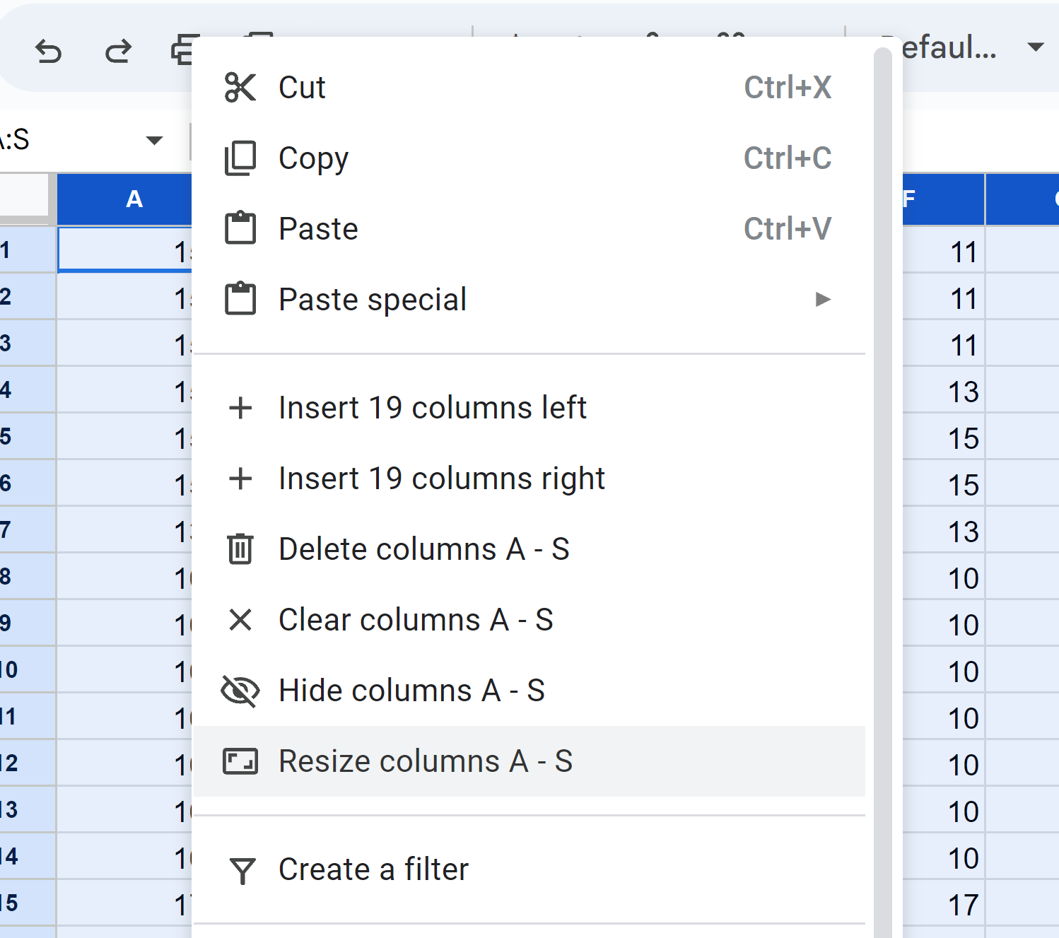 Picture of resizing columns in Google Sheets
Do the same for the rows, specifying 30px for each.
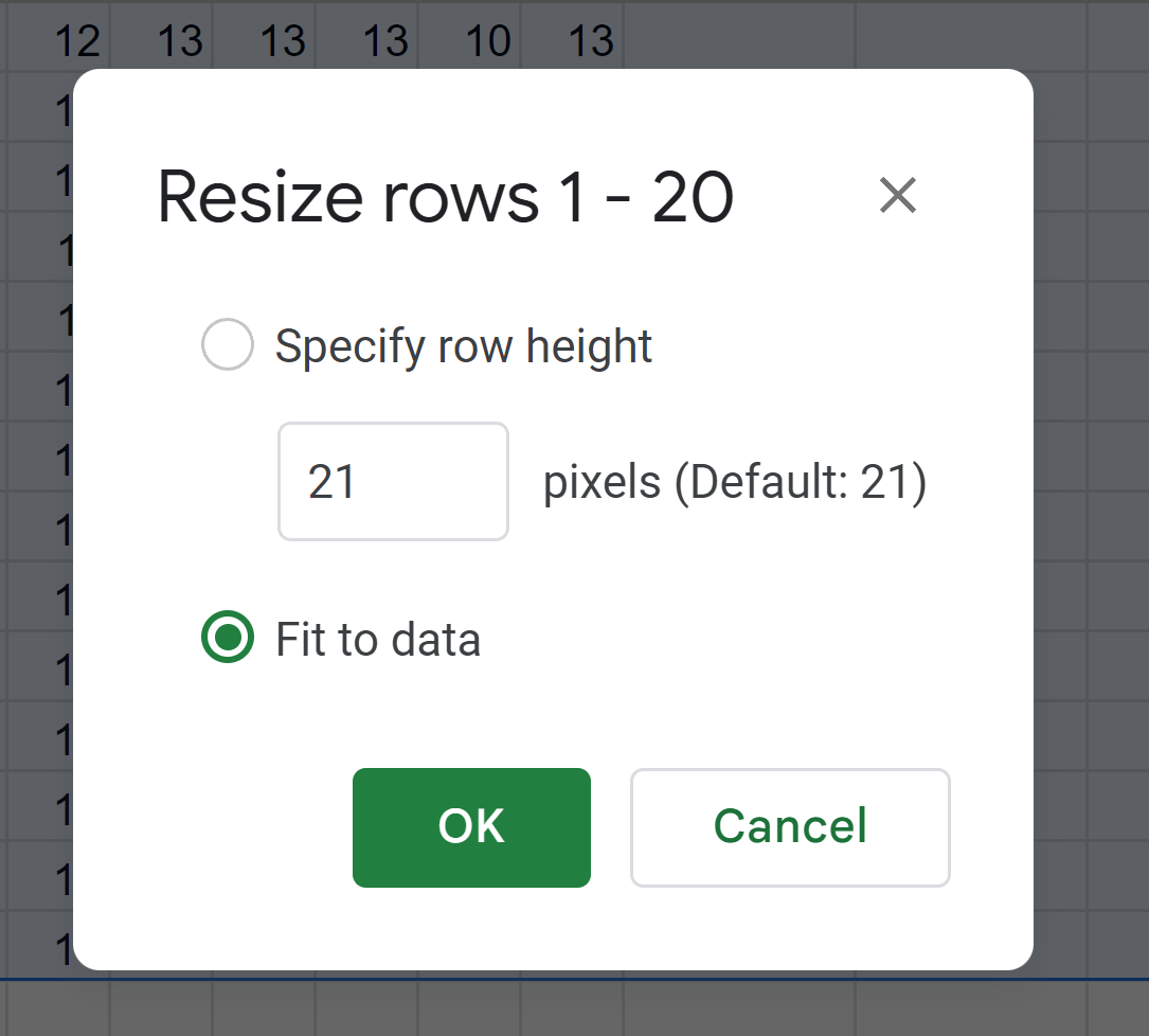 Picture of resizing rows in Google Sheets
Turn off the gridlines by selecting View -> Show -> Gridlines.
 Picture of View options in Google Sheets
Conditional Formatting
Select the entire range where all the numbers are and then click Format -> Conditional formatting.
Click Add new rule and under Format rules, select Is equal to from the dropdown menu.
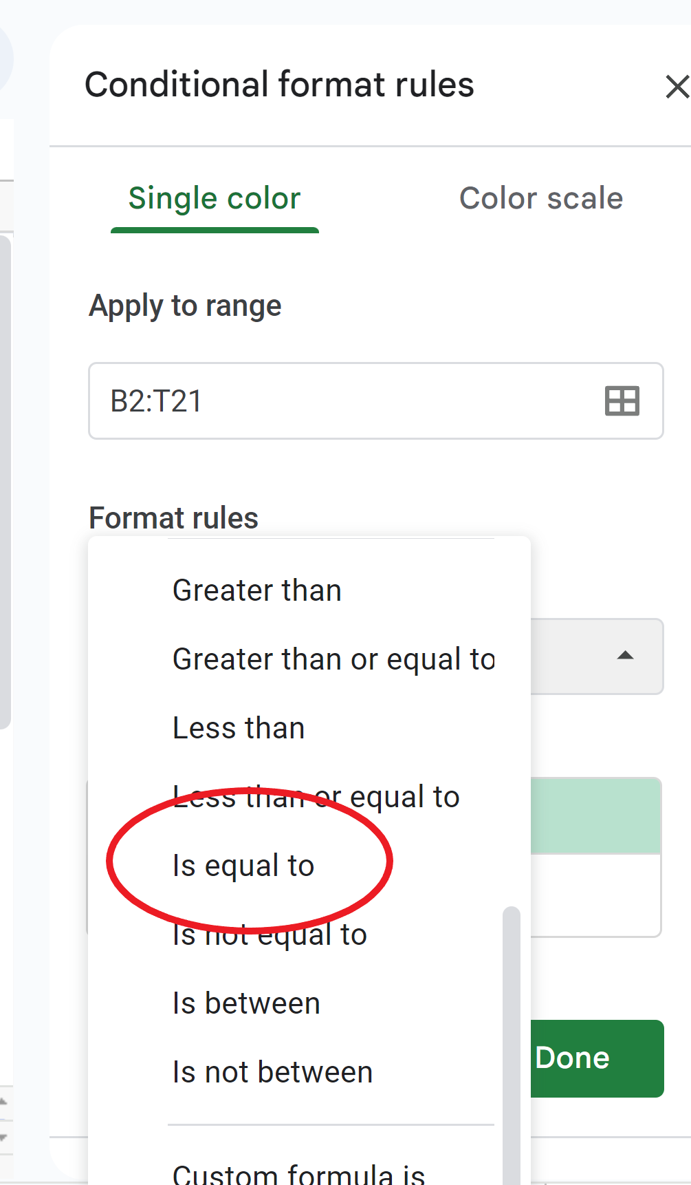 Picture of conditional formatting in Google Sheets
Under Formatting style, follow the color key from the coloring page you selected and adjust the font and background colors according to each number.
In our example, all the number 10s need to be blue, so we enter 10 and then have the same blue for both background and font colors:
 Picture of color options in Google Sheets
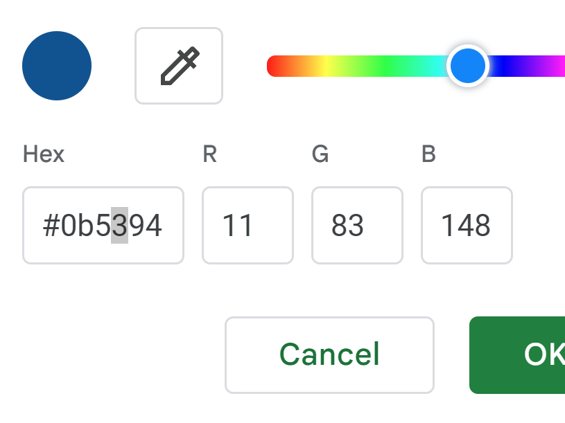
⭐Important Note
Because of the script we're writing and how we're triggering it, you need to alter the HEX code for one of these two numbers. If they are the exact same, it will cause an error later.
So, first enter the same color for both, then open one and select the plus icon in the custom color swatch.
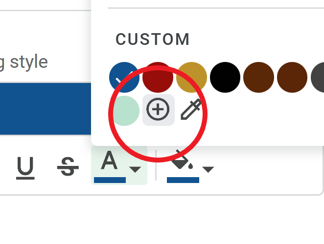 Picture of custom colors in Google Sheets
Manually change one value in the HEX code by one digit. In the example, I changed it from #0b5294 to #0b5394. Visually, it will still look the same. If this is confusing, be sure to check out the walkthrough video at 02:39.
 Picture of custom colors in Google Sheets
Do this for each color in your piece of art, and you'll have a gorgeous piece of pixel artwork in your spreadsheet. This alone is rewarding! 😀
 Picture of volcano pixel art in Google Sheets
Apps Script Setup
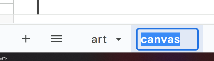
Name the sheet that we're on by double clicking Sheet1 at the bottom. We'll call it "art". Then make a new sheet by clicking the plus icon on the bottom bar. Name it "canvas".
 Picture of sheet names in Google Sheets
Setup the canvas in the same way we did at the beginning, only without the conditional formatting. Make everything the same size, remove the gridlines, and add a border around the B2:T21 range that will serve as a frame.
Now, we need to make buttons to toggle in each cell. In Google Sheets, the way to do this is by adding checkboxes to all the cells. Checkboxes will hold either a true or false value, and when we click them, they'll change back and forth.
Select our full range again, and select Data -> Data validation. Change the criteria to Checkbox and under Advanced options select Reject the input.
 Picture of data validation rules in Google Sheets
This will give our script something to be triggered by.
Format these checkboxes in the same way we did our conditional formatting: make the background white: #ffffff, and the font color just slightly different: #fffeff. Then, give them a huge font size, like 200. This will allow for us to click anywhere in the cell and not run the risk of clicking just outside the border of the box itself.
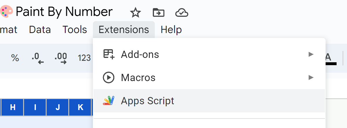
Now, let's open our code editor by selecting Extensions -> Apps Script.
 Picture of Extensions menu in Google Sheets
Script Logic
We need to copy and paste the formatting of individual cells every time we click the blank cells in our canvas.
To do this, we'll use an onEdit(e) trigger method built into Apps Script.
function onEdit(e) {
  //get current sheet
  var sheet = SpreadsheetApp.getActiveSheet();

  // if we're not on the art sheet...
  if(sheet.getName() != "art"){
First, we'll grab the active sheet as a variable. Then, making sure we're not on the "art" sheet, we'll go through the steps to grab and paste the formatting we need...
// get the active cell and it's row, column reference
var activeRange = sheet.getActiveCell();
var row = activeRange.getRow();
var column = activeRange.getColumn();
Within our conditional if statement, we'll make three more variables so that we can grab the position of the cell we're in.
Then we need to go to our "art" sheet and grab the formatting from the corresponding cell.
var artRange = SpreadsheetApp.getActive().getSheetByName("art").getRange(row,column);
// get the background color from the same reference in art sheet
var backgroundColor = artRange.getBackground();
var fontColor = artRange.getFontColor();
We'll make another three variables: one for the artRange which grabs the range from the "art" sheet using the row and column that we're on in the "canvas" sheet. And then two variables for the colors: one for background and one for font.
Now all we need to do is set the "canvas" sheet's cell to the colors we just grabbed. I've also chosen to make it toggle back to a blank white cell if it's already been colored. So we'll use another if statement to handle that:
trueFalse = activeRange.getValue();
if(trueFalse){
      // set activeRange with that backgroundColor
      activeRange.setBackground(backgroundColor);
      activeRange.setFontColor(fontColor);
    }
    else{
      activeRange.setBackground('#ffffff');
      activeRange.setFontColor('#fffeff');
    }
First, we set a trueFalse variable equal to the activeRange's value. This is either true or false depending on the state of the checkbox.
If it's false (the checkbox isn't checked), then we set the background and font colors using the variables we grabbed from our "art" sheet.
Here's the full onEdit(e) code:
function onEdit(e) {
  //get current sheet
  var sheet = SpreadsheetApp.getActiveSheet();

  // if we're not on the art sheet...
  if(sheet.getName() != "art"){

    // get the active cell and it's row, column reference
    var activeRange = sheet.getActiveCell();
    var row = activeRange.getRow();
    var column = activeRange.getColumn();

    var artRange = SpreadsheetApp.getActive().getSheetByName("art").getRange(row,column);

    // get the background color from the same reference in art sheet
    var backgroundColor = artRange.getBackground();
    var fontColor = artRange.getFontColor();

    Logger.log(backgroundColor)
    Logger.log(fontColor)

    trueFalse = activeRange.getValue();

    if(trueFalse){
      // set activeRange with that backgroundColor
      activeRange.setBackground(backgroundColor);
      activeRange.setFontColor(fontColor);
    }
    else{
      activeRange.setBackground('#ffffff');
      activeRange.setFontColor('#fffeff');
    }
  }
}
Reset Function
As an added feature, we'll add an actual button to reset the canvas. To do this, we'll make a new function in our Apps Script code editor.
We'll grab the sheet and all the checkboxes as variables. To get the checkboxes, we'll use the getRangebyName() method on our 'canvasArt' range.
Then, Apps Script makes it pretty easy with built in methods. We set the value of all the checkboxes to false, the background color to #ffffff, and the font color to #fffeff.
Here's the full reset() code:
function reset(){
  var sheet = SpreadsheetApp.getActive();
  var checkboxes = sheet.getRangeByName('canvasArt');
  checkboxes.setValue(false);
  checkboxes.setBackground("#ffffff");
  checkboxes.setFontColor("#fffeff");
}
Trigger with Button
To make a button in the spreadsheet, select Insert -> Drawing.
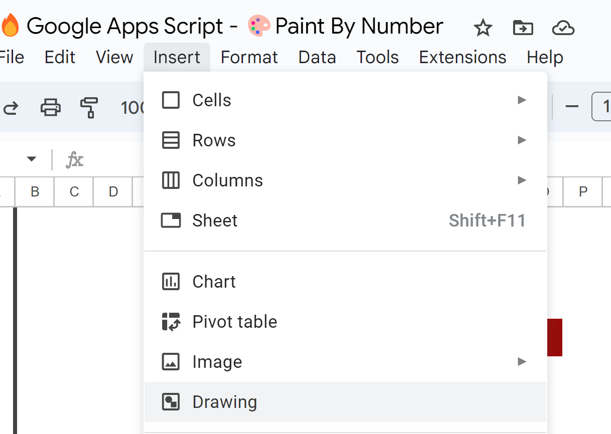 Picture of Insert menu in Google Sheets
Select the rounded rectangle shape and drag it onto the grid.
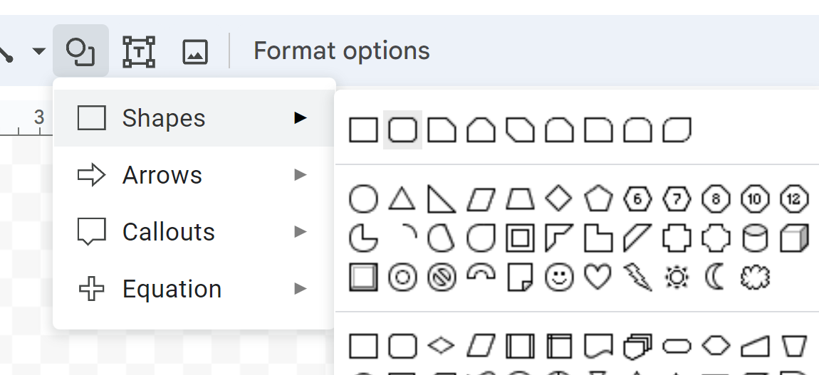 Picture of Shapes menu in Google Sheets
Double click into the shape to write "CLEAR". Adjust the font and colors as you see fit.
 Picture of button drawing in Google Sheets
Click Save and Close and then drag it to re-size and reposition onto your sheet at the bottom of the canvas.
Once you've positioned it, click the three circles in the top right, select Assign script, and type in the name of the script you'd like it to trigger (in our case, reset).
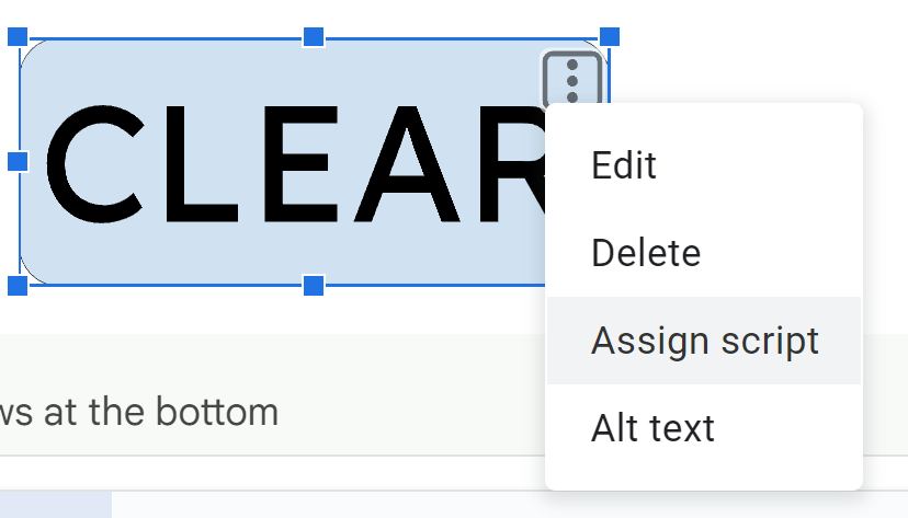 Picture of assigning script to button in Google Sheets
Now, when you click this button, that script will run and clear the whole art canvas.
Conclusion
I hope this has been helpful for you! I had a great time making this, and I have more game-type spreadsheet content coming soon.
Come follow me on YouTube, and say hey over on LinkedIn.
Have a great one! 👋