
By Björn Hartmann
When reading articles about machine learning, I often suspect that authors misunderstand the term “linear model.” Many authors suggest that linear models can only be applied if data can be described with a line. But this is way too restrictive.
Linear models assume the functional form is linear — not the relationship between your variables.
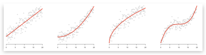
I’ll show you how you can improve your linear regressions with quadratic, root, and exponential functions.
So what’s the functional form?
The functional form is the equation you want to estimate.
Let us start with an example and think about how we could describe salaries of data scientists. Suppose an average data scientist (i) receives an entry-level salary (entry_level_salary) plus a bonus for each year of his experience (experience_i).
Thus, his salary (salary_i) is given by the following functional form:
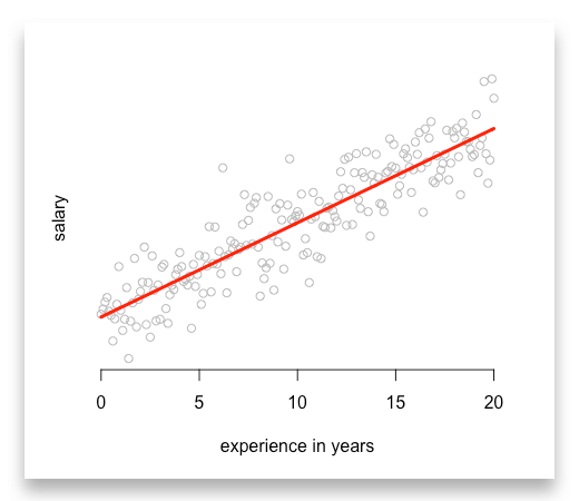
salary_i = entry_level_salary + beta_1 * experience_i
Now, we can interpret the coefficient beta_1 as the bonus for each year of experience. And with this coefficient we can start making predictions by just knowing the level of experience.
As your machine learning model takes care of the coefficient beta_1 , all you need to enter in R or any other software is:
model_1 <- lm(salary ~ entry_level_salary + experience)
Linearity in the functional form requires that we sum up each determinant on the right-hand side of the equation.
Imagine we are right with our assumptions. Each point indicates one data scientist with his level of experience and salary. Finally, the red line is our predictions.
Many aspiring data scientists already run similar predictions. But often that is all they do with linear models…
How to estimate quadratic models?
When we want to estimate a quadratic model, we cannot type in something like this:
model_2 <- lm(salary ~ entry_level_salary + experience^2)
>> This will reject an error message
Most of these functions do not expect that they have to transform your input variables. As a result, they reject an error message if you try. Furthermore, you do not have a sum at the right-hand side of the equation anymore.
Note: You need to compute experience^² before adding it into your model. Thus, you will run:
# First, compute the square values of experienceexperience_2 <- experience^2
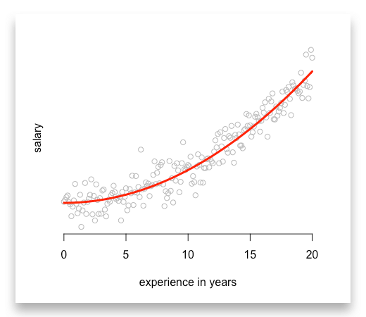
# Then add them into your regressionmodel_2 <- lm(salary ~ entry_level_salary + experience_2)
In return, you get a nice quadratic function:
Estimate root functions with linear models
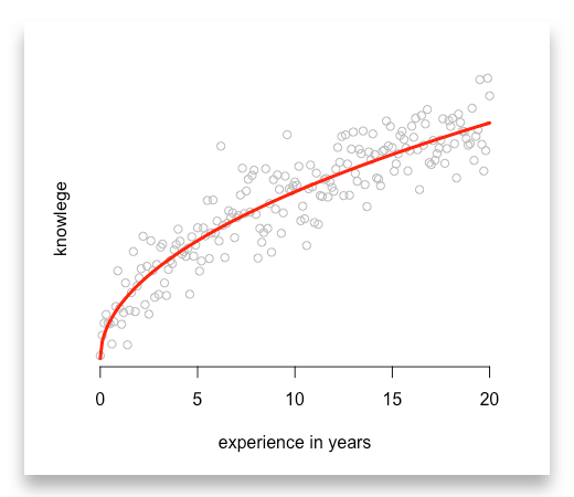
Often we observe values that rise fast in the beginning and align to certain level afterwards. Let us modify our example and estimate a typical learning curve.
In the beginning a learning curve tends to be very steep and slows down after some years.
There is one function that features such a trend, the root function. So we use the square root of experience to capture this relationship:
# First, compute the square root values of experiencesqrt_experience <- sqrt(experience)
# Then add them into your regressionmodel_3 <- lm(knowledge ~ sqrt_experience)
Again, make sure you compute the square root before you add it to your model:
Or you might want to use the logarithmic function as it describes a similar trend. But its’ values are negative between zero and one. So make sure this is not a problem for you and your data.
Mastering linear models
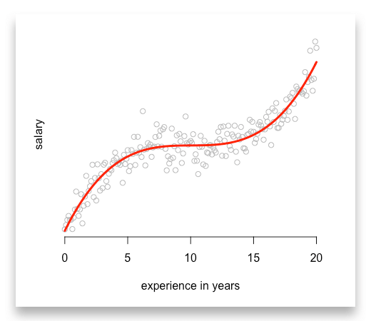
Finally, you can even estimate polynomial functions with higher orders or exponential functions. All you need to do is to compute all variables before you add them into your linear model:
# First, compute polynomialsexperience_2 <- experience^2experience_3 <- experience^3
# Then add them into your regressionmodel_4 <- lm(salary ~ experience + experience_2 + experience_3)
Two cases where you should use other models
Although linear models can be applied to many cases, there are limitations. The most popular can be divided into two categories:
1. Probabilities:
If you want to estimate the probability of an event, you better use Probit, Logit or Tobit models. When estimating probabilities you use distributions that linear functions cannot capture. Depending on the distribution you assume, you should choose between the Probit, Logit or Tobit model.
2. Count variables
Finally, when estimating a count variable you want to use a Poisson model. Count variables are variable that can only be integers such as 1, 2, 3, 4.
For example count the number of children, the number of purchases a customer makes or the number of accidents in a region.
What to take away from this article
There are two things I want you to remember:
- Improve your linear models and try quadratic, root or polynomial functions.
- Always transform your data before you add them to your regression.
I uploaded the R code for all examples on GitHub. Feel free to download them, play with them, or share them with your friends and colleagues.

If you have any questions, write a comment below or contact me. I appreciate your feedback.