
By Björn Hartmann
Find out which linear regression model is the best fit for your data
Inspired by a question after my previous article, I want to tackle an issue that often comes up after trying different linear models: You need to make a choice which model you want to use. More specifically, Khalifa Ardi Sidqi asked:
“How to determine which model suits best to my data? Do I just look at the R square, SSE, etc.?
As the interpretation of that model (quadratic, root, etc.) will be very different, won’t it be an issue?”
The second part of the question can be answered easily. First, find a model that best suits to your data and then interpret its results. It is good if you have ideas how your data might be explained. However, interpret the best model, only.
The rest of this article will address the first part of his question. Please note that I will share my approach on how to select a model. There are multiple ways, and others might do it differently. But I will describe the way that works best for me.
In addition, this approach only applies to univariate models. Univariate models have just one input variable. I am planning a further article, where I will show you how to assess multivariate models with more input variables. For today, however, let us focus on the basics and univariate models.
To practice and get a feeling for this, I wrote a small ShinyApp. Use it and play around with different datasets and models. Notice how parameters change and become more confident with assessing simple linear models. Finally, you can also use the app as a framework for your data. Just copy it from Github.
Use the Adjusted R2 for univariate models
If you only use one input variable, the adjusted R2 value gives you a good indication of how well your model performs. It illustrates how much variation is explained by your model.
In contrast to the simple R2, the adjusted R2 takes the number of input factors into account. It penalizes too many input factors and favors parsimonious models.
In the screenshot above, you can see two models with a value of 71.3 % and 84.32%. Apparently, the second model is better than the first one. Models with low values, however, can still be useful because the adjusted R2 is sensitive to the amount of noise in your data. As such, only compare this indicator of models for the same dataset than comparing it across different datasets.
Usually, there is little need for the SSE
Before you read on, let’s make sure we are talking about the same SSE. On Wikipedia, SSE refers to the sum of squared errors. In some statistic textbooks, however, SSE can refer to the explained sum of squares (the exact opposite). So for now, suppose SSE refers to the sum of squared errors.
Hence, the adjusted R2 is approximately 1 — SSE /SST. With SST referring to the total sum of squares.
I do not want to dive deeper into the math behind this. What I want to show you is that the adjusted R2 is computed with the SSE. So the SSE usually does not give you any additional information.
Furthermore, the adjusted R2 is normalized such that it is always between zero and one. So it is easier for you and others to interpret an unfamiliar model with an adjusted R2 of 75% rather than an SSE of 394 — even though both figures might explain the same model.
Have a look at the residuals or error terms!
What is often ignored are error terms or so-called residuals. They often tell you more than what you might think.
The residuals are the difference between your predicted values and the actual values.
Their benefit is that they can show you both the magnitude as well as the direction of your errors. Let’s have a look at an example:
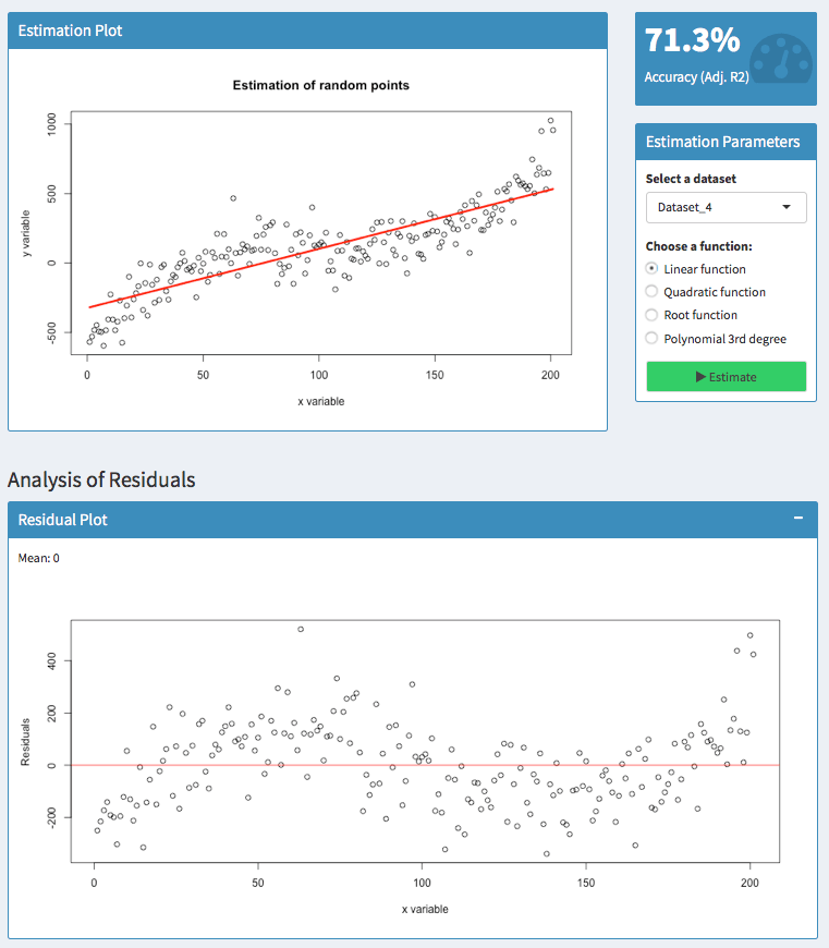
Here, I tried to predict a polynomial dataset with a linear function. Analyzing the residuals shows that there are areas where the model has an upward or downward bias.
For 50 &l_t_; x < 100, the residuals are above zero. So in this area, the actual values have been higher than the predicted values — our model has a downward bias.
For100 < x < 150, however, the residuals are below zero. Thus, the actual values have been lower than the predicted values — the model has an upward bias.
It is always good to know, whether your model suggests too high or too low values. But you usually do not want to have patterns like this.
The residuals should be zero on average (as indicated by the mean) and they should be equally distributed. Predicting the same dataset with a polynomial function of 3 degrees suggests a much better fit:
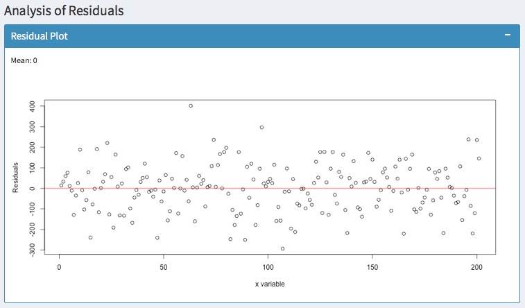
In addition, you can observe whether the variance of your errors increases. In statistics, this is called Heteroscedasticity. You can fix this easily with robust standard errors. Otherwise, your hypothesis tests are likely to be wrong.
Histogram of residuals
Finally, the histogram summarizes the magnitude of your error terms. It provides information about the bandwidth of errors and indicates how often which errors occurred.
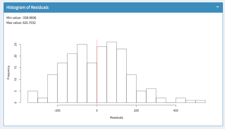
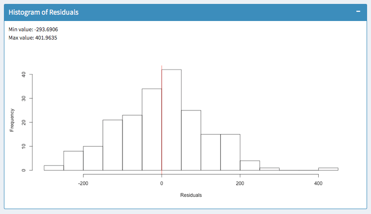
The above screenshots show two models for the same dataset. In the left histogram, errors occur within a range of -338 and 520.
In the right histogram, errors occur within -293 and 401. So the outliers are much lower. Furthermore, most errors in the model of the right histogram are closer to zero. So I would favor the right model.
Summary
When choosing a linear model, these are factors to keep in mind:
- Only compare linear models for the same dataset.
- Find a model with a high adjusted R2
- Make sure this model has equally distributed residuals around zero
- Make sure the errors of this model are within a small bandwidth

If you have any questions, write a comment below or contact me. I appreciate your feedback.