

I’m an AI researcher, so one of the main things I deal with is data. A lot of it.
With more than 2.5 exabytes of data generated every day, it comes as no surprise that this data needs to be stored somewhere where we can access it when we need it.
This article will walk you through a hackable cheatsheet to get you up and running with SQL quickly.
What is SQL?
SQL stands for Structured Query Language. It is a language for relational database management systems. SQL is used today to store, retrieve, and manipulate data within relational databases.
Here’s what a basic relational database looks like:

Using SQL, we can interact with the database by writing queries.
Here’s what an example query looks like:
SELECT * FROM customers;
Using this SELECT statement, the query selects all the data from all the columns in the customer’s table and returns data like so:
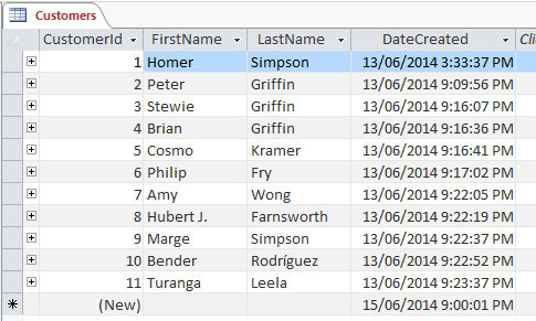
Source: Database Guide
The asterisk wildcard character (*) refers to “all” and selects all the rows and columns. We can replace it with specific column names instead — here only those columns will be returned by the query
SELECT FirstName, LastName FROM customers;
Adding a WHERE clause allows you to filter what gets returned:
SELECT * FROM customers WHERE age >= 30 ORDER BY age ASC;
This query returns all data from the products table with an age value of greater than 30.
The use of ORDER BY keyword just means the results will be ordered using the age column from the lowest value to the highest
Using the INSERT INTO statement, we can add new data to a table. Here’s a basic example adding a new user to the customers table:
INSERT INTO customers(FirstName, LastName, address, email)
VALUES ('Alice', 'Bob', 'McLaren Vale, South Australia', 'test@fakeGmail.com');
Of course, these examples demonstrate only a very small selection of what the SQL language can do. We'll learn more about it in this guide.
Why Learn SQL?
We live in the age of Big Data, where data is used extensively to find insights and inform strategy, marketing, advertising and a plethora of other operations.
Big businesses like Google, Amazon, AirBnb utilize large, relational databases as a basis of improving customer experience. Understanding SQL is a great skill to have not only for data scientists and analysts but for everyone.
How do you think that you suddenly got a Youtube ad on shoes when just a few minutes ago, you were Googling your favourite shoes? That’s SQL (or a form of SQL) at work!
SQL vs MySQL
Before we move on, I just want to clarify an often-confused topic — the difference between SQL and MySQL. As it turns out, they aren’t the same thing!
SQL is a language, while MySQL is a system to implement SQL.
SQL outlines syntax that allows you to write queries that manage relational databases.
MySQL is a database system that runs on a server. It allows you to write queries using SQL syntax to manage MySQL databases.
In addition to MySQL, there are other systems that implement SQL. Some of the more popular ones include:
SQLite
Oracle Database
PostgreSQL
Microsoft SQL Server
How to Install MySQL
For most cases, MySQL is the preferred choice for a database management system. Many popular Content Management Systems (like Wordpress) use MySQL by default, so using MySQL to manage those applications can be a good idea.
In order to use MySQL, you’ll need to install it on your system:
Install MySQL on Windows
The recommended way to install MySQL on Windows is by using the MSI installer from the MySQL website.
This resource will guide you with the installation process.
Install MySQL on macOS
On macOS, installing MySQL also involves downloading an installer.
This resource will guide you through the installation process.
How to Use MySQL
With MySQL now installed on your system, I recommend that you use some sort of SQL management application to make managing your databases a much easier process.
There are lots of apps to choose from which largely do the same job, so it’s down to your own personal preference on which one to use:
MySQL Workbench developed by Oracle
phpMyAdmin (operates in the web browser)
HeidiSQL (Recommended for Windows)
Sequel Pro (Recommended for macOS)
When you’re ready to start writing your own SQL queries, consider importing dummy data rather than creating your own database.
Here are some dummy databases that are available for download free of charge.
SQL Cheatsheet – The Icing on the Cake
SQL Keywords
Here you can find a collection of keywords used in SQL statements, a description, and where appropriate an example. Some of the more advanced keywords have their own dedicated section.
Where MySQL is mentioned next to an example, this means this example is only applicable to MySQL databases (as opposed to any other database system).
ADD -- Adds a new column to an existing table

ADD CONSTRAINT -- Creates a new constraint on an existing table, which is used to specify rules for any data in the table.

ALTER TABLE -- Adds, deletes or edits columns in a table. It can also be used to add and delete constraints in a table, as per the above.

ALTER COLUMN -- Changes the data type of a table’s column.

ALL -- Returns true if all of the subquery values meet the passed condition.

AND -- Used to join separate conditions within a WHERE clause.

ANY -- Returns true if any of the subquery values meet the given condition.

AS -- Renames a table or column with an alias value which only exists for the duration of the query.

ASC -- Used with ORDER BY to return the data in ascending order.

BETWEEN -- Selects values within the given range.

CASE -- Changes query output depending on conditions.

CHECK -- Adds a constraint that limits the value which can be added to a column.

CREATE DATABASE -- Creates a new database.

CREATE TABLE -- Creates a new table.

DEFAULT -- Sets a default value for a column

DELETE -- Delete data from a table.

DESC -- Used with ORDER BY to return the data in descending order.

DROP COLUMN -- Deletes a column from a table.

DROP DATABASE -- Deletes the entire database.

DROP DEAFULT -- Removes a default value for a column.

DROP TABLE -- Deletes a table from a database.

EXISTS -- Checks for the existence of any record within the subquery, returning true if one or more records are returned.

FROM -- Specifies which table to select or delete data from.

IN --  Used alongside a WHERE clause as a shorthand for multiple OR conditions.

INSERT INTO -- Adds new rows to a table.

IS NULL -- Tests for empty (NULL) values.

IS NOT NULL -- The reverse of NULL. Tests for values that aren’t empty / NULL.

LIKE -- Returns true if the operand value matches a pattern.

NOT -- Returns true if a record DOESN’T meet the condition.

OR -- Used alongside WHERE to include data when either condition is true.

ORDER BY -- Used to sort the result data in ascending (default) or descending order through the use of ASC or DESC keywords.

ROWNUM -- Returns results where the row number meets the passed condition.

SELECT -- Used to select data from a database, which is then returned in a results set.

SELECT DISTINCT -- Sames as SELECT, except duplicate values are excluded.

SELECT INTO -- Copies data from one table and inserts it into another.

SELECT TOP -- Allows you to return a set number of records to return from a table.

SET -- Used alongside UPDATE to update existing data in a table.

SOME -- Identical to ANY.

TOP -- Used alongside SELECT to return a set number of records from a table.

TRUNCATE TABLE -- Similar to DROP, but instead of deleting the table and its data, this deletes only the data.

UNION -- Combines the results from 2 or more SELECT statements and returns only distinct values.

UNION ALL -- The same as UNION, but includes duplicate values.

UNIQUE -- This constraint ensures all values in a column are unique.

UPDATE -- Updates existing data in a table.

VALUES -- Used alongside the INSERT INTO keyword to add new values to a table.

WHERE -- Filters results to only include data which meets the given condition.
Comments in SQL
Comments allow you to explain sections of your SQL statements, without being executed directly.
In SQL, there are 2 types of comments, single line and multiline.
Single Line Comments in SQL
Single line comments start with ‘- -’. Any text after these 2 characters to the end of the line will be ignored.
-- This part is ignored

SELECT * FROM customers;
Multiline Comments in SQL
Multiline comments start with /* and end with */. They stretch across multiple lines until the closing characters have been found.
/*

This is a multiline comment.
It can span across multiple lines.

*/

SELECT * FROM customers;

/*

This is another comment.
You can even put code within a comment to prevent its execution

SELECT * FROM icecreams;

*/
Data Types in MySQL
When creating a new table or editing an existing one, you must specify the type of data that each column accepts.
In this example, data passed to the id column must be an int (integer), while the FirstName column has a VARCHAR data type with a maximum of 255 characters.
CREATE TABLE customers(
id int,
FirstName varchar(255)
);
1. String Data Types
CHAR(size) -- Fixed length string which can contain letters, numbers and special characters. The size parameter sets the maximum string length, from 0 – 255 with a default of 1.

VARCHAR(size) -- Variable length string similar to CHAR(), but with a maximum string length range from 0 to 65535.

BINARY(size) -- Similar to CHAR() but stores binary byte strings.

VARBINARY(size) -- Similar to VARCHAR() but for binary byte strings.

TINYBLOB -- Holds Binary Large Objects (BLOBs) with a max length of 255 bytes.

TINYTEXT -- Holds a string with a maximum length of 255 characters. Use VARCHAR() instead, as it’s fetched much faster.

TEXT(size) -- Holds a string with a maximum length of 65535 bytes. Again, better to use VARCHAR().

BLOB(size) -- Holds Binary Large Objects (BLOBs) with a max length of 65535 bytes.

MEDIUMTEXT -- Holds a string with a maximum length of 16,777,215 characters.

MEDIUMBLOB -- Holds Binary Large Objects (BLOBs) with a max length of 16,777,215 bytes.

LONGTEXT -- Holds a string with a maximum length of 4,294,967,295 characters.

LONGBLOB -- Holds Binary Large Objects (BLOBs) with a max length of 4,294,967,295 bytes.

ENUM(a, b, c, etc…) -- A string object that only has one value, which is chosen from a list of values which you define, up to a maximum of 65535 values. If a value is added which isn’t on this list, it’s replaced with a blank value instead.

SET(a, b, c, etc…) -- A string object that can have 0 or more values, which is chosen from a list of values which you define, up to a maximum of 64 values.
2. Numeric Data Types
BIT(size) -- A bit-value type with a default of 1. The allowed number of bits in a value is set via the size parameter, which can hold values from 1 to 64.

TINYINT(size) -- A very small integer with a signed range of -128 to 127, and an unsigned range of 0 to 255. Here, the size parameter specifies the maximum allowed display width, which is 255.

BOOL -- Essentially a quick way of setting the column to TINYINT with a size of 1. 0 is considered false, whilst 1 is considered true.

BOOLEAN    -- Same as BOOL.

SMALLINT(size) -- A small integer with a signed range of -32768 to 32767, and an unsigned range from 0 to 65535. Here, the size parameter specifies the maximum allowed display width, which is 255.

MEDIUMINT(size) -- A medium integer with a signed range of -8388608 to 8388607, and an unsigned range from 0 to 16777215. Here, the size parameter specifies the maximum allowed display width, which is 255.

INT(size) -- A medium integer with a signed range of -2147483648 to 2147483647, and an unsigned range from 0 to 4294967295. Here, the size parameter specifies the maximum allowed display width, which is 255.

INTEGER(size) -- Same as INT.

BIGINT(size) -- A medium integer with a signed range of -9223372036854775808 to 9223372036854775807, and an unsigned range from 0 to 18446744073709551615. Here, the size parameter specifies the maximum allowed display width, which is 255.

FLOAT(p) -- A floating point number value. If the precision (p) parameter is between 0 to 24, then the data type is set to FLOAT(), whilst if it's from 25 to 53, the data type is set to DOUBLE(). This behaviour is to make the storage of values more efficient.

DOUBLE(size, d) -- A floating point number value where the total digits are set by the size parameter, and the number of digits after the decimal point is set by the d parameter.

DECIMAL(size, d) -- An exact fixed point number where the total number of digits is set by the size parameters, and the total number of digits after the decimal point is set by the d parameter.

DEC(size, d) -- Same as DECIMAL.
3. Date/Time Data Types
DATE -- A simple date in YYYY-MM–DD format, with a supported range from ‘1000-01-01’ to ‘9999-12-31’.

DATETIME(fsp) -- A date time in YYYY-MM-DD hh:mm:ss format, with a supported range from ‘1000-01-01 00:00:00’ to ‘9999-12-31 23:59:59’. By adding DEFAULT and ON UPDATE to the column definition, it automatically sets to the current date/time.

TIMESTAMP(fsp) -- A Unix Timestamp, which is a value relative to the number of seconds since the Unix epoch (‘1970-01-01 00:00:00’ UTC). This has a supported range from ‘1970-01-01 00:00:01’ UTC to ‘2038-01-09 03:14:07’ UTC.
By adding DEFAULT CURRENT_TIMESTAMP and ON UPDATE CURRENT TIMESTAMP to the column definition, it automatically sets to current date/time.

TIME(fsp) -- A time in hh:mm:ss format, with a supported range from ‘-838:59:59’ to ‘838:59:59’.

YEAR -- A year, with a supported range of ‘1901’ to ‘2155’.
SQL Operators
1. Arithmetic Operators in SQL
+ -- Add
– -- Subtract
* -- Multiply
/ -- Divide
% -- Modulus
2. Bitwise Operators in SQL
& -- Bitwise AND
| -- Bitwise OR
^-- Bitwise XOR
3. Comparison Operators in SQL
= -- Equal to
> -- Greater than
< -- Less than
>= -- Greater than or equal to
<= -- Less than or equal to
<> -- Not equal to
4. Compound Operators in SQL
+= -- Add equals
-= -- Subtract equals
*= -- Multiply equals
/= -- Divide equals
%= -- Modulo equals
&= -- Bitwise AND equals
^-= -- Bitwise exclusive equals
|*= -- Bitwise OR equals
SQL Functions
1. String Functions in SQL
ASCII -- Returns the equivalent ASCII value for a specific character.

CHAR_LENGTH -- Returns the character length of a string.

CHARACTER_LENGTH -- Same as CHAR_LENGTH.

CONCAT -- Adds expressions together, with a minimum of 2.

CONCAT_WS -- Adds expressions together, but with a separator between each value.

FIELD -- Returns an index value relative to the position of a value within a list of values.

FIND IN SET -- Returns the position of a string in a list of strings.

FORMAT -- When passed a number, returns that number formatted to include commas (eg 3,400,000).

INSERT -- Allows you to insert one string into another at a certain point, for a certain number of characters.

INSTR -- Returns the position of the first time one string appears within another.

LCASE -- Converts a string to lowercase.

LEFT -- Starting from the left, extracts the given number of characters from a string and returns them as another.

LENGTH -- Returns the length of a string, but in bytes.

LOCATE -- Returns the first occurrence of one string within another,

LOWER -- Same as LCASE.

LPAD -- Left pads one string with another, to a specific length.

LTRIM -- Removes any leading spaces from the given string.

MID -- Extracts one string from another, starting from any position.

POSITION -- Returns the position of the first time one substring appears within another.

REPEAT -- Allows you to repeat a string

REPLACE -- Allows you to replace any instances of a substring within a string, with a new substring.

REVERSE    -- Reverses the string.

RIGHT -- Starting from the right, extracts the given number of characters from a string and returns them as another.

RPAD -- Right pads one string with another, to a specific length.

RTRIM -- Removes any trailing spaces from the given string.

SPACE -- Returns a string full of spaces equal to the amount you pass it.

STRCMP -- Compares 2 strings for differences

SUBSTR -- Extracts one substring from another, starting from any position.

SUBSTRING -- Same as SUBSTR

SUBSTRING_INDEX    -- Returns a substring from a string before the passed substring is found the number of times equals to the passed number.

TRIM --    Removes trailing and leading spaces from the given string. Same as if you were to run LTRIM and RTRIM together.

UCASE -- Converts a string to uppercase.

UPPER -- Same as UCASE.
2. Numeric Functions in SQL
ABS -- Returns the absolute value of the given number.

ACOS -- Returns the arc cosine of the given number.

ASIN -- Returns the arc sine of the given number.

ATAN -- Returns the arc tangent of one or 2 given numbers.

ATAN2 -- Returns the arc tangent of 2 given numbers.

AVG -- Returns the average value of the given expression.

CEIL -- Returns the closest whole number (integer) upwards from a given decimal point number.

CEILING -- Same as CEIL.

COS -- Returns the cosine of a given number.

COT -- Returns the cotangent of a given number.

COUNT -- Returns the amount of records that are returned by a SELECT query.

DEGREES -- Converts a radians value to degrees.

DIV -- Allows you to divide integers.

EXP -- Returns e to the power of the given number.

FLOOR -- Returns the closest whole number (integer) downwards from a given decimal point number.

GREATEST -- Returns the highest value in a list of arguments.

LEAST -- Returns the smallest value in a list of arguments.

LN -- Returns the natural logarithm of the given number.

LOG -- Returns the natural logarithm of the given number, or the logarithm of the given number to the given base.

LOG10 -- Does the same as LOG, but to base 10.

LOG2 -- Does the same as LOG, but to base 2.

MAX -- Returns the highest value from a set of values.

MIN -- Returns the lowest value from a set of values.

MOD -- Returns the remainder of the given number divided by the other given number.

PI -- Returns PI.

POW -- Returns the value of the given number raised to the power of the other given number.

POWER -- Same as POW.

RADIANS -- Converts a degrees value to radians.

RAND -- Returns a random number.

ROUND -- Rounds the given number to the given amount of decimal places.

SIGN -- Returns the sign of the given number.

SIN -- Returns the sine of the given number.

SQRT -- Returns the square root of the given number.

SUM -- Returns the value of the given set of values combined.

TAN -- Returns the tangent of the given number.

TRUNCATE -- Returns a number truncated to the given number of decimal places.
3. Date Functions in SQL
ADDDATE -- Adds a date interval (eg: 10 DAY) to a date (eg: 20/01/20) and returns the result (eg: 20/01/30).

ADDTIME -- Adds a time interval (eg: 02:00) to a time or datetime (05:00) and returns the result (07:00).

CURDATE -- Gets the current date.

CURRENT_DATE -- Same as CURDATE.

CURRENT_TIME -- Gest the current time.

CURRENT_TIMESTAMP -- Gets the current date and time.

CURTIME -- Same as CURRENT_TIME.

DATE -- Extracts the date from a datetime expression.

DATEDIFF -- Returns the number of days between the 2 given dates.

DATE_ADD -- Same as ADDDATE.

DATE_FORMAT -- Formats the date to the given pattern.

DATE_SUB -- Subtracts a date interval (eg: 10 DAY) to a date (eg: 20/01/20) and returns the result (eg: 20/01/10).

DAY -- Returns the day for the given date.

DAYNAME -- Returns the weekday name for the given date.

DAYOFWEEK -- Returns the index for the weekday for the given date.

DAYOFYEAR -- Returns the day of the year for the given date.

EXTRACT -- Extracts from the date the given part (eg MONTH for 20/01/20 = 01).

FROM DAYS -- Returns the date from the given numeric date value.

HOUR -- Returns the hour from the given date.

LAST DAY -- Gets the last day of the month for the given date.

LOCALTIME -- Gets the current local date and time.

LOCALTIMESTAMP -- Same as LOCALTIME.

MAKEDATE -- Creates a date and returns it, based on the given year and number of days values.

MAKETIME -- Creates a time and returns it, based on the given hour, minute and second values.

MICROSECOND -- Returns the microsecond of a given time or datetime.

MINUTE -- Returns the minute of the given time or datetime.

MONTH -- Returns the month of the given date.

MONTHNAME -- Returns the name of the month of the given date.

NOW -- Same as LOCALTIME.

PERIOD_ADD -- Adds the given number of months to the given period.

PERIOD_DIFF -- Returns the difference between 2 given periods.

QUARTER -- Returns the year quarter for the given date.

SECOND -- Returns the second of a given time or datetime.

SEC_TO_TIME -- Returns a time based on the given seconds.

STR_TO_DATE -- Creates a date and returns it based on the given string and format.

SUBDATE -- Same as DATE_SUB.

SUBTIME -- Subtracts a time interval (eg: 02:00) to a time or datetime (05:00) and returns the result (03:00).

SYSDATE -- Same as LOCALTIME.

TIME -- Returns the time from a given time or datetime.

TIME_FORMAT -- Returns the given time in the given format.

TIME_TO_SEC -- Converts and returns a time into seconds.

TIMEDIFF -- Returns the difference between 2 given time/datetime expressions.

TIMESTAMP -- Returns the datetime value of the given date or datetime.

TO_DAYS -- Returns the total number of days that have passed from ‘00-00-0000’ to the given date.

WEEK -- Returns the week number for the given date.

WEEKDAY -- Returns the weekday number for the given date.

WEEKOFYEAR -- Returns the week number for the given date.

YEAR -- Returns the year from the given date.

YEARWEEK -- Returns the year and week number for the given date.
4. Miscellaneous Functions in SQL
BIN -- Returns the given number in binary.

BINARY -- Returns the given value as a binary string.

CAST -- Converst one type into another.

COALESCE -- From a list of values, returns the first non-null value.

CONNECTION_ID -- For the current connection, returns the unique connection ID.

CONV -- Converts the given number from one numeric base system into another.

CONVERT -- Converts the given value into the given datatype or character set.

CURRENT_USER -- Returns the user and hostname which was used to authenticate with the server.

DATABASE -- Gets the name of the current database.

GROUP BY -- Used alongside aggregate functions (COUNT, MAX, MIN, SUM, AVG) to group the results.

HAVING -- Used in the place of WHERE with aggregate functions.

IF -- If the condition is true it returns a value, otherwise it returns another value.

IFNULL -- If the given expression equates to null, it returns the given value.

ISNULL -- If the expression is null, it returns 1, otherwise returns 0.

LAST_INSERT_ID -- For the last row which was added or updated in a table, returns the auto increment ID.

NULLIF -- Compares the 2 given expressions. If they are equal, NULL is returned, otherwise the first expression is returned.

SESSION_USER -- Returns the current user and hostnames.

SYSTEM_USER -- Same as SESSION_USER.

USER -- Same as SESSION_USER.

VERSION -- Returns the current version of the MySQL powering the database.
Wildcard Characters in SQL
In SQL, Wildcards are special characters used with the LIKE and NOT LIKE keywords. This allows us to search for data with sophisticated patterns rather efficiently.
% -- Equates to zero or more characters.
-- Example: Find all customers with surnames ending in ‘ory’.
SELECT * FROM customers
WHERE surname LIKE '%ory';

_ -- Equates to any single character.
-- Example: Find all customers living in cities beginning with any 3 characters, followed by ‘vale’.
SELECT * FROM customers
WHERE city LIKE '_ _ _vale';

[charlist] -- Equates to any single character in the list.
-- Example: Find all customers with first names beginning with J, K or T.
SELECT * FROM customers
WHERE first_name LIKE '[jkt]%';
SQL Keys
In relational databases, there is a concept of primary and foreign keys. In SQL tables, these are included as constraints, where a table can have a primary key, a foreign key, or both.
1. Primary Keys in SQL
A primary lets each record in a table be uniquely identified. You can only have one primary key per table, and you can assign this constraint to any single or combination of columns. However, this means each value within this column(s) needs to be unique.
Typically in a table, the ID column is a primary key, and is usually paired with the AUTO_INCREMENT keyword. This means the value increases automatically as and when new records are created.
Example (MySQL)
Create a new table and set the primary key to the ID column.
CREATE TABLE customers (
id int NOT NULL AUTO_INCREMENT,
FirstName varchar(255),
Last Name varchar(255) NOT NULL,
address varchar(255),
email varchar(255),
PRIMARY KEY (id)
);
2. Foreign Keys in SQL
You can apply a foreign key to one column or many. You use it to link 2 tables together in a relational database.
The table containing the foreign key is called the child key,
The table containing the referenced (or candidate) key is called the parent table.
This essentially means that the column data is shared between 2 tables, because a foreign key also prevents invalid data from being inserted which isn’t also present in the parent table.
Example (MySQL)
Create a new table and turn any column that references IDs in other tables into foreign keys.
CREATE TABLE orders (
id int NOT NULL,
user_id int,
product_id int,
PRIMARY KEY (id),
FOREIGN KEY (user_id) REFERENCES users(id),
FOREIGN KEY (product_id) REFERENCES products(id)
);
Indexes in SQL
Indexes are attributes that can be assigned to columns that are frequently searched against to make data retrieval a quicker and more efficient process.
CREATE INDEX -- Creates an index named ‘idx_test’ on the first_name and surname columns of the users table. In this instance, duplicate values are allowed.
CREATE INDEX idx_test
ON users (first_name, surname);
CREATE UNIQUE INDEX -- The same as the above, but no duplicate values.
CREATE UNIQUE INDEX idx_test
ON users (first_name, surname);
DROP INDEX -- Removes an index.
ALTER TABLE users
DROP INDEX idx_test;
SQL Joins
In SQL, a JOIN clause is used to return a result which combines data from multiple tables, based on a common column which is featured in both of them.
There are a number of different joins available for you to use:
Inner Join (Default): Returns any records which have matching values in both tables.
Left Join: Returns all of the records from the first table, along with any matching records from the second table.
Right Join: Returns all of the records from the second table, along with any matching records from the first.
Full Join: Returns all records from both tables when there is a match.
A common way of visualising how joins work is like this:

Source: Website Setup
SELECT orders.id, users.FirstName, users.Surname, products.name as ‘product name’
FROM orders
INNER JOIN users on orders.user_id = users.id
INNER JOIN products on orders.product_id = products.id;
Views in SQL
A view is essentially an SQL results set that gets stored in the database under a label, so you can return to it later without having to rerun the query.
These are especially useful when you have a costly SQL query which you might need a number of times. So instead of running it over and over to generate the same results set, you can just do it once and save it as a view.
How to Create Views in SQL
To create a view, you can do so like this:
CREATE VIEW priority_users AS
SELECT * FROM users
WHERE country = ‘United Kingdom’;
Then in future, if you need to access the stored result set, you can do so like this:
SELECT * FROM [priority_users];
How to Replace Views in SQL
With the CREATE OR REPLACE command, you can update a view like this:
CREATE OR REPLACE VIEW [priority_users] AS
SELECT * FROM users
WHERE country = ‘United Kingdom’ OR country=’USA’;
How to Delete Views in SQL
To delete a view, simply use the DROP VIEW command.
DROP VIEW priority_users;
Conclusion
The majority of websites and applications use relational databases in some way or the other. This makes SQL extremely valuable to know as it allows you to create more complex, functional systems.
Happy learning!