By Patrick Ferris
Learning the “TensorFlow way” to build a neural network can seem like a big hurdle to getting started with machine learning. In this tutorial, we’ll take it step by step and explain all of the critical components involved as we build a Bands2Vec model using Pitchfork data from Kaggle.
For the full code, check out the GitHub page.
The Word2Vec Model
Neural networks consume numbers and produce numbers. They’re very good at it. But give them some text, and they’ll throw a tantrum and do nothing remotely interesting.
If it is the neural network’s job to crunch the numbers and produce meaningful output, then it is our job to make sure that whatever we are feeding it is meaningful too. This quest for a meaningful representation of information gave birth to the Word2Vec model.
One approach to working with words is to form one-hot encoded vectors. Create a long (the number of distinct words in our vocabulary) list of zeroes, and have each word point to a unique index of this list. If we see this word, make that index in the list a number one.
While this approach works, it requires a lot space and is completely devoid of meaning. ‘Good’ and ‘Excellent’ are as similar as ‘Duck’ and ‘Blackhole’. If only there was a way to vectorise words so that we preserved this contextual similarity…
Thankfully, there is a way!
Using a neural network, we can produce ‘embeddings’ of our words. These are vectors that represent each unique word extracted from the weights of the connections within our network.
But the question remains: how do we make sure they’re meaningful? The answer: feed in pairs of words as a target word and a context word. Do this enough times, throwing in some bad examples too, and the neural network begins to learn what words appear together and how this forms almost a graph. Like a social network of words interconnected by contexts. ‘Good’ goes to ‘helpful’ which goes to ‘caring’ and so on. Our task is to feed this data into the neural network.
One of the most common approaches is the Skipgram model, generating these target-context pairings based on moving a window across a dataset of text. But what if our data isn’t sentences, but we still have contextual meaning?
In this tutorial, our words are artist names and our contexts are genres and mean review scores. We want artist A to be close to artist B if they share a genre and have a mean review score that is similar. So let’s get started.
Building our Dataset
Pitchfork is an online American music magazine covering mostly rock, independent, and new music. The data released to Kaggle was scraped from their website and contains information like reviews, genres, and dates linked to each artist.
Let’s create an artist class and dictionary to store all of the useful information we want.
Great! Now we want to manufacture our target-context pairings based on genre and mean review score. To do this, we’ll create two dictionaries: one for the different unique genres, and one for the scores (discretised to integers).
We’ll add all our artists to the corresponding genre and mean score in these dictionaries to use later when generating pairs of artists.
One last step before we dive into the TensorFlow code: generating a batch! A batch is like a sample of data that our neural network will use for each epoch. An epoch is one sweep across the neural network in a training phase. We want to generate two numpy arrays. One will contain the following code:
TensorFlow
There are a myriad of TensorFlow tutorials and sources of knowledge out there. Any of these excellent articles will help you as well as the documentation. The following code is heavily based on the word2vec tutorial from the TensorFlow people themselves. Hopefully I can demystify some of it and boil it down to the essentials.
The first step is understanding the ‘graph’ representation. This is incredibly useful for the TensorBoard visualisations and for creating a mental image of the data flows within the neural network.
Take some time to read through the code and comments below. Before we feed data to a neural network, we have to initialise all of the parts we’re going to use. The placeholders are the inputs taking whatever we give the ‘feed_dict’. The variables are mutable parts of the graph that we will eventually tweak. The most important part of our model is the loss function. It’s the score of how well we did and the treasure map to how we can improve.
Noise Contrastive Estimation (NCE) is a loss function. Usually we would use cross-entropy and softmax, but in the natural language processing world, all of our classes amount to every single unique word.
Computationally, this is bad. NCE changes the framing of the problem from probabilities of classes to whether or not a target-context pairing is correct (a binary classification). It takes a true pairing and then samples to get bad pairings, the constant num_sampled controls this. Our neural network learns to distinguish between these good and bad pairings. Ultimately, it learns the contexts! You can read more about NCE and how it works here.
Run the Neural Network
Now that everything is set up nicely, we just have to hit the big green ‘go’ button and twiddle our thumbs for a bit.
Visualization using TSNE
Okay, we’re not quite done. We now have context-rich, 64-dimensional vectors for our artists, but that’s perhaps too many dimensions to really visualize its usefulness.
Lucky for us we can squash this information into two dimensions while retaining as many of the properties as the 64 dimensions had! This is T-distributed Stochastic Neighbor Embedding, or TSNE for short. This video does a great job of explaining the main idea behind TSNE, but I’ll try to give a broad overview.
TSNE is an approach to dimensionality reduction that retains the similarities (like Euclidean distance) of higher dimensions. To do this, it first builds a matrix of point-to-point similarities calculated using a normal distribution. The centre of the distribution is the first point, and the similarity of the second point is the value of the distribution at the distance between the points away from the centre of the distribution.
Then we project randomly onto the dimension below and do exactly the same process using a t-distribution. Now we have two matrices of point-to-point similarities. The algorithm then slowly moves the points in the lower dimension to try and make it look like the matrix for the higher dimension where the similarities were preserved. And repeat. Thankfully, Sci-kit Learn has a function which can do the number crunching for us.
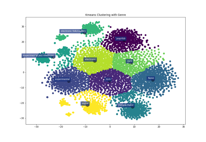
The Results
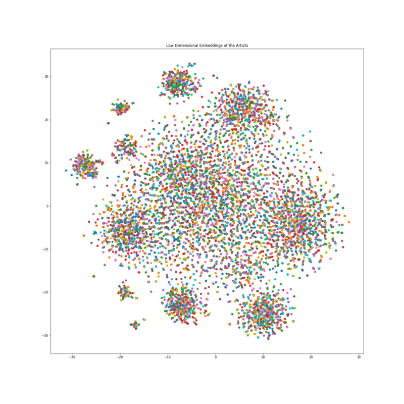 All of the Artists plotted using their low dimensional embedding
The amazing aspect of these embeddings is that, just like vectors, they support mathematical operations. The classic example being: King — Man + Woman = Queen , or at least very close to it. Let’s try an example.
Take the low dimensional embeddings of Coil, a band with the following genres, [‘electronic’, ‘experimental', ‘rock’] , and mean score 7.9. Now subtract the low dimensional embeddings of Elder Ones, a band with genres,['electronic'] , and mean score 7.8. With this embedding difference, find the closest bands to it and print their names and genres.
Artist: black lips, Mean Score: 7.48, Genres: ['rock', 'rock', 'rock', 'rock', 'rock']
Artist: crookers, Mean Score: 5.5, Genres: ['electronic']
Artist: guided by voices, Mean Score: 7.23043478261, Genres: ['rock', 'rock', 'rock', 'rock', 'rock', 'rock', 'rock', 'rock', 'rock', 'rock', 'rock', 'rock', 'rock', 'rock', 'rock', 'rock', 'rock', 'rock', 'rock', 'rock', 'rock', 'rock', 'rock']
It worked! We’re getting rock and electronic bands with vaguely similar review scores. Below are the first three hundred bands plotted with labels. Hopefully you’ve found this project educational and inspiring. Go forth and build, explore, and play!
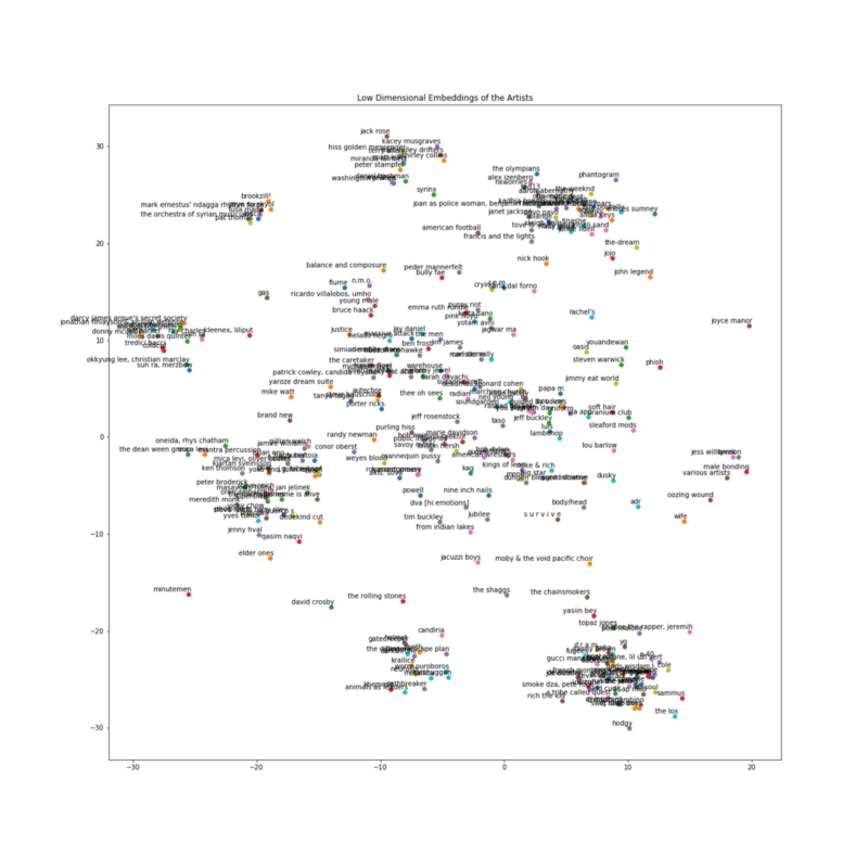 Three hundred artists plotted and labelled