
There are several ways to lookup data in a spreadsheet. If you're building a dashboard, you'll find this very useful.
The =XLOOKUP() function is my new favorite way to lookup data. It's discussed in the last section 👇.
We'll look at four of the built in lookup functions in both Excel and Google Sheets:
=LOOKUP()=VLOOKUP()=HLOOKUP()=XLOOKUP()
Now, if you've spent any time in spreadsheets, you've probably heard mention of or are already using =VLOOKUP(). It is one of the most popular functions out there, but is also a bit mystifying if you don't use it on a regular basis.
🏆 I'll walkthrough each of these to give you a full understanding of how to use the functions properly. And I'll highlight my new favorite, =XLOOKUP(), that Microsoft released in 2019 and Google Sheets added in 2022.
☕ I've also built a coffee themed Google Sheet that you can open and follow along with. Here it is.
📽️ And, I've got you covered...at the end of the article there's a video walkthrough too. 💥
 Gif of athlete pointing and saying, I Got You!
Coffee Data
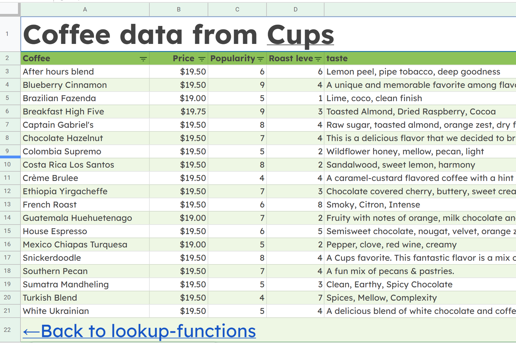
In our coffee data spreadsheet, I have made two sheets with the same data on it. One, the coffee-data tab, is for LOOKUP and VLOOKUP. The horizontal-data tab is for HLOOKUP.
Here's what the coffee-data tab looks like. There are columns for the coffee name, price, popularity, roast level and taste.
 Coffee Data Spreadsheet Screenshot
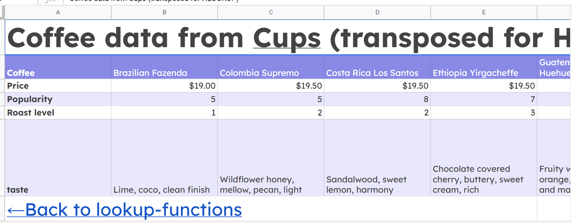
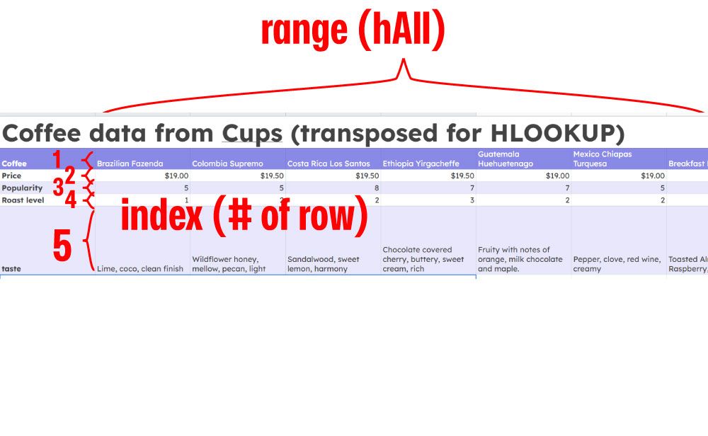
Here's what the horizontal-data tab looks like. Same info, just transposed so we can walk through the HLOOKUP function in a bit.
 Coffee Data Horizontal Spreadsheet Screenshot
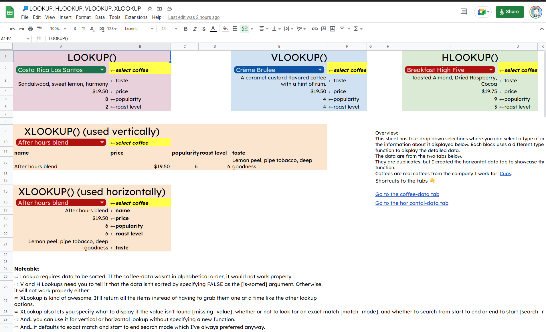
And then we have our main tab, lookup-functions, where we'll examine the different functions below.
If you haven't pulled up the Google Sheet yet, go ahead so you can follow along: https://docs.google.com/spreadsheets/d/1rNAJKwGQzdq8F2zMrAwHMQvY_z3FlBs9BIy_4MIOXn4/edit#gid=1137792422
Everything works the same in Excel, but it's very easy to share Google Sheets. You can make your own copy to work in by clicking File -> Make a copy.
I've created several named ranges in this sheet to make it easier as we fill out the functions. You can examine those by clicking Data -> Named ranges. I'll reference these in the function definitions below.
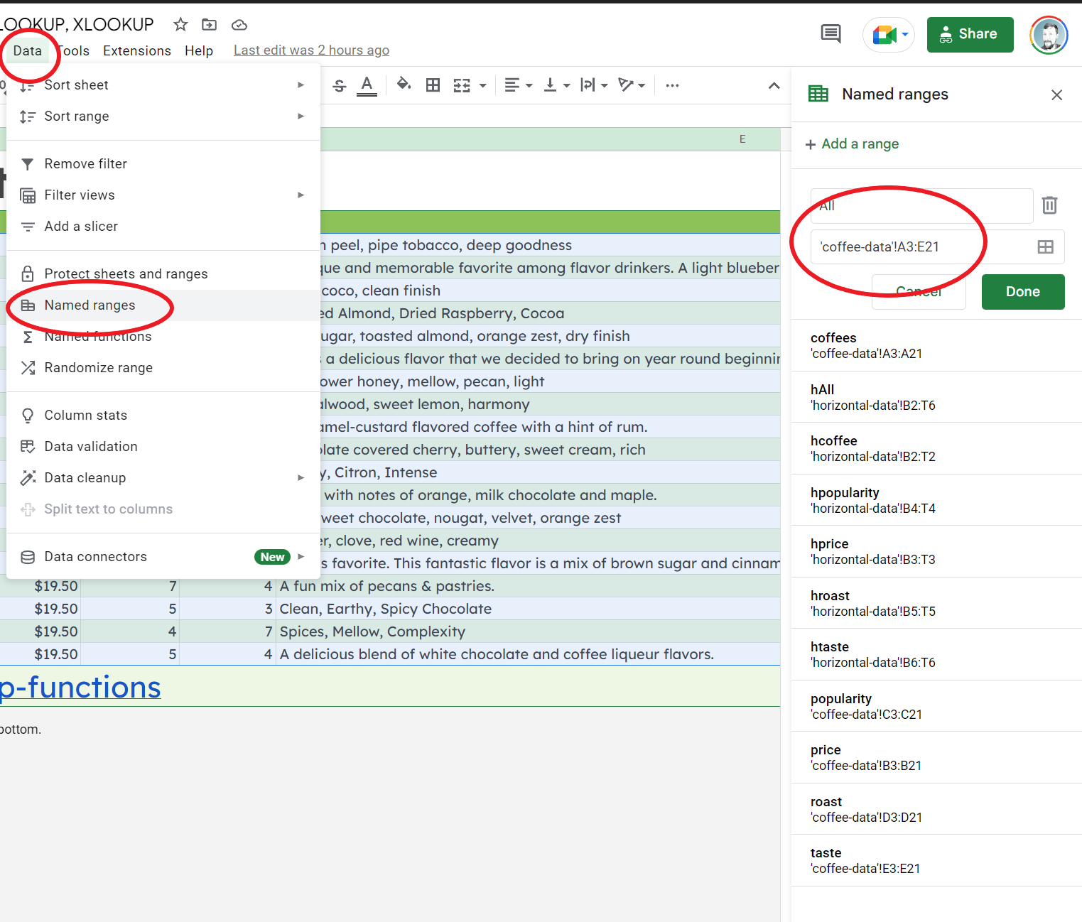 Screenshot of named ranges in Google Sheets
How to Use the LOOKUP Function
No surprise here – =LOOKUP() lets you look up a value in your data. Same as everything else here.
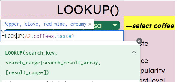
Here's our LOOKUP function to return the taste: =LOOKUP(A2,coffees,taste).
We're using named ranges (coffees & taste) which define the coffees column and the tasting notes column in our coffee-data.
If you pull up the sample Google Sheet, you'll see that we're giving LOOKUP three arguments: the search_key, search_range|search_result_array, and the optional [result_range].
 Screenshot of Lookup function
The search_key is the thing we're searching for. In our example, it's the name of the coffee we want information about. All of the functions have a search_key argument.
The search_range|search_result_array is the range where =LOOKUP() needs to find the search_key. It can be used as both search and result ranges too.
Say you have search keys in your coffee column (A) and the result you want displayed is the taste column (E). If you specify A:E as the search_range|search_result_array then you'll get the tasting notes on whatever coffee you're searching for.
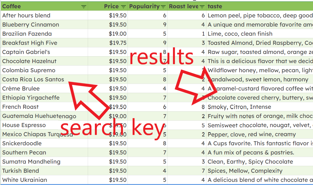 Screenshot of table of data
When you do this, the result range value will come from the last column (or row) in the range.
The alternative is to simply specify the search_range column on the coffee column and then enter another range for the result_range.
This is what I've done in our sample spreadsheet since I wanted to pull data from each of the columns about the coffee.
Shortcomings of =LOOKUP():
- Data must be sorted. It will not work properly if it's not.
- You must specify the single return column or row for the result.
How to Use the VLOOKUP Function
This is a very popular function because it lets you lookup data with a little more power than the regular LOOKUP function.
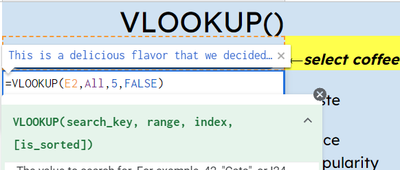
Here's our VLOOKUP function to return the taste: =VLOOKUP(E2,All,5,FALSE).
We're using another named range. This time, just one is needed. We have All which is the entire table of coffee-data.
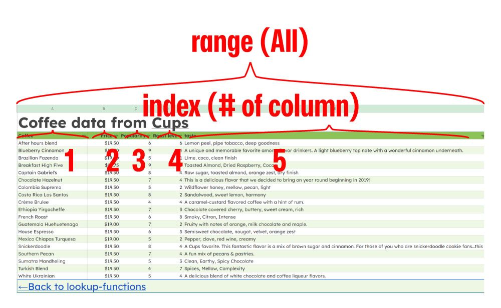 Screenshot of table of data
With =VLOOKUP() we enter the search_key as before but then we give it a range to search. The first column in the range will be used to find the search_key. Then we give it an index which tells how many columns to the right we want to look for our returned value.
We then type in FALSE to indicate that our data isn't sorted. (This is actually unnecessary here since we sorted it so that the regular LOOKUP function would work properly).
 Screenshot of VLookup function
Shortcomings of =VLOOKUP():
- Must lookup data from left to right.
- Must specify a number for the index. If you add or move columns in your data, you risk breaking the formula.
- Defaults to sorted data. In many cases, you'll need to set that argument as
FALSEso the function will work properly.
How to User the HLOOKUP Function
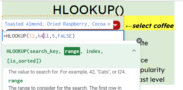
HLOOKUP works basically the same as VLOOKUP except that instead of searching through columns, it searches through rows.
Here's our HLOOKUP function to return the taste: =HLOOKUP(I2,hAll,5,FALSE)
 Screenshot of table of horizontal data
Check out the horizontal-data tab to see that I've transposed the same data set so that our search_key now is spread across a row instead of down a column. Then when we give an index value, it returns that value by counting from top to bottom:
 Screenshot of HLookup function
So if we wanted the price, we'd have index of 2 since it's the second row down. And in our example, we return taste with an index of 5.
Shortcomings are the same as VLOOKUP.
How to Use the XLOOKUP Function
Enter: =XLOOKUP()! Microsoft released this as a successor to VLOOKUP and HLOOKUP in 2019, and Google Sheets finally added it in August of 2022.
What's different?
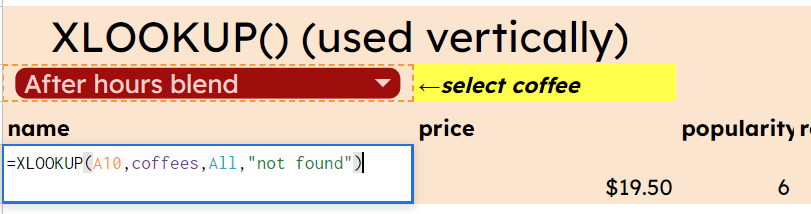
Well, to start with, you can use it vertically or horizontally. You don't have to specify one or the other as long as you have the proper ranges as arguments.
Check out both of the XLOOKUP blocks on the sample spreadsheet. One is using it as a vertical lookup and the second as a horizontal lookup. All that is necessary are that the ranges are correct: The search_key must be a single row or column, and the lookup_range must be of the same size depending on which is used.
 Screenshot of XLookup function used vertically
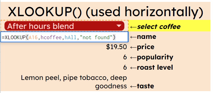 Screenshot of XLookup function used horizontally
Some more features/advantages:
=XLOOKUP()defaults to an exact match so you don't have to specify amatch_modeif this is what you're after.- You're able to define a custom string to display as
missing_valueinstead of#N/Ain the event that nothing is returned. - You're able to define
search_modeto search from the last entry to the first if you desire. InVLOOKUPandHLOOKUP, it is only possible to go first to last. - Instead of declaring new functions for each desired value (
price,popularity,roast level, andtaste),=XLOOKUP()will return each value in the givenlookup_range.
If you want don't want all the values returned, you'd need to reduce the size of the range.
In the spreadsheet example, I've defined my ranges All and hAll to include all the columns and rows, respectively. If I wanted to leave out taste, for instance, we'd need to leave that column/row out of the lookup_range.
=XLOOKUP() was introduced to be the successor of =VLOOKUP() and =HLOOKUP. I think I'll be using it going forward, what about you?
Conclusion
As with most things in computer programming and spreadsheets, there are many ways to solve the same problem.
We've explored four ways to lookup data in a spreadsheet: =LOOKUP(), =VLOOKUP(), =HLOOKUP() and =XLOOKUP(). Each is powerful, but =XLOOKUP(), the newest function, is particularly useful in combining and expanding many features of its predecessors.
Here is a video walkthrough of everything we've discussed:
Thanks🙏for reading and watching!
Subscribe🔔to my YouTube channel here: https://www.youtube.com/@EamonnCottrell/
And say hey👋on LinkedIn here: https://www.linkedin.com/in/eamonncottrell/