Machine Learning Basics for Developers

In the current tech landscape, developers are expected to have a number of different skills. And many of them do.

There are also a lot of different career paths available to developers that use many of their current skills with a slight twist.

Database administrators, developer advocates, and machine learning engineers all have one thing in common with all developers: they all know how to code. It doesn't matter which languages are being used, they all understand the core concepts behind writing good code.

That's one of the reasons many software developers consider becoming machine learning engineers. With all of the tools and packages available, you don't need to have a deep mathematical background to get accurate results.

If you are willing to learn how to use some libraries and get a high-level understanding of the underlying math, you can become a machine learning engineer.

In this article, I'll walk you through the some of the main concepts in machine learning that you need to understand coming from a software developer background.

We'll end with an example of an entire machine learning project, from getting data to predicting a value with a model. By the end, you should have enough knowledge to complete a small machine learning project of your own from scratch.

What is machine learning?

There are a lot of definitions out there. But machine learning basically involves using math to find patterns in massive amounts of data to make predictions based on new data.

Once it has found those patterns, you can say that you have a machine learning model.

From there you can use the model to make predictions on new data that the model has never seen before.

The goal is to get computers to automatically improve with experience using the algorithms they're provided.

An algorithm is just a math equation or a set of equations that give you a result based on your input data. Machine learning uses algorithms to find those patterns we're looking for.

As the algorithms get exposed to more and more data, they start to make more accurate predictions. Eventually the model built by the algorithms will be able to figure out the correct result without being explicitly programmed to do so.

This means that the computer should be able to take in data and make decisions (predictions) without any human help.

Machine learning vs. data science vs. artificial intelligence

Many people use the terms machine learning, data science, and artificial intelligence interchangeably. But they are not the same things.

Machine learning is used in data science to make predictions and discover patterns in your data.

Data science focuses more on statistics and algorithms and the interpretation of results. Machine learning is focused more on the software and automation of things.

Artificial intelligence refers to a computer's ability to understand and learn from data, while making decisions based on hidden patterns that would be almost impossible for humans to figure out.

Machine learning is like a branch of artificial intelligence. We'll use machine learning to achieve artificial intelligence.

Artificial intelligence is a broad topic, and it covers things like computer vision, human-computer interactions, and autonomy where machine learning would be used in each of those applications.

Different types of machine learning

There are three types of machine learning you'll hear and read about: supervised learning, semi-supervised learning, and unsupervised learning.

Supervised learning

This is the category most machine learning problems fall under. It's when you have input and output variables and you're trying to make a mapping between them.

It's called supervised learning because we can use the data to teach the model the right answer.

The algorithm will make predictions based on the data and it will slowly be corrected until those predictions match the output that's expected.

Most of the problems supervised learning covers can be solved with classification or regression. As long as you have labeled data, you're working with supervised machine learning.

Semi-supervised learning

Most real world problems fall into this area because of our data sets.

In many cases you'll have a large data set where some of the data is labeled, but most of it isn't. Sometimes it can be too expensive to have an expert go through and label all of this data, so you use a blend of supervised and unsupervised learning.

One strategy is using the labeled data to make guesses about the unlabeled data, and then using those predictions as their labels. Then you can use all of the data in some kind of supervised learning model.

Since it's possible to do unsupervised learning on these data sets as well, consider if that would be a more efficient way to go.

Unsupervised learning

When you only have input data and no associated output data and you want a model to make the pattern you're looking for, that's when you enter unsupervised learning.

Your algorithm is going to make something up that makes sense to it based on the parameters you give it.

This is useful when you have a lot of seemingly random data and you want to see if there are any interesting patterns in them. These problems are usually great for clustering algorithms and give you some unexpected results.

Practical uses of machine learning for developers

Classification

When you want to predict a label for a some input data, this is a classification problem.

Machine learning handles classification by building a model that takes data that's already been labeled and uses it to make predictions on new data. Basically you give it a new input and it gives you the label it thinks is correct.

Predicting customer churn, face classification, and medical diagnostic tests all use different kinds of classification.

While all of these fall under different domains of classification, they all assign values based on the data their models used for training. All of the predicted values are exact. So you'll predict values like a name or a Boolean.

Regression

Regression is interesting because it crosses over machine learning and statistics. It's similar to classification because it's used to predict values, except it predicts continuous values instead of discrete values.

So if you want to predict a salary range based on years of experience and languages known, or you want to predict a house price based on location and square footage, you would be handling a regression problem.

There are different regression techniques to handle all kinds of data sets, even non-linear data.

There's support vector regression, simple linear regression, and polynomial regression among many others. There are enough regression techniques out there to fit just about any data set you have.

Clustering

This moves into a different type of machine learning. Clustering handles unsupervised learning tasks. It's like classification, but none of the data is labeled. It's up to the algorithm to find and label data points.

This is great when you have a massive data set and you don't know of any patterns between them, or you're looking for uncommon connections.

Clustering helps when you want to find anomalies and outliers in your data without spending hundreds of hours manually labeling data points.

In this case, there's often not a best algorithm and the best way to find what works for your data is through testing different algorithms.

A few clustering algorithms include: K-Means, DBSCAN, Agglomerative Clustering, and Affinity Propagation. Some trial and error will help you quickly find what algorithm is the most efficient for you.

Deep learning

This is a field of machine learning that uses algorithms inspired by how the brain works. It involves neural networks using large unclassified data sets.

Typically performance improves with the amount of data you feed a deep learning algorithm. These types of problems deal with unlabeled data which covers the majority of data available.

There are a number of algorithms you can use with this technique, like Convolutional Neural Networks, Long Short-Term Memory Networks, or the Deep Q-Network.

Each of these are used in projects like computer vision, autonomous vehicles, or analyzing EEG signals.

Tools you might use

There are a number of tools available that you can use for just about any machine learning problem you have.

Here's a short list of some of the common packages you'll find in many machine learning applications.

Pandas: This is a general data analysis tool in Python. It helps when you need to work with raw data. It handles textual data, tabular data, time series data, and more.

This package is used to format data before training a machine learning model in many cases.

Tensorflow: You can build any number of machine learning applications with this library. You can run it on GPUs, use it to solve IoT problems, and it's great for deep learning.

This is the library that can handle just about anything, but it takes some time to get up to speed with it.

SciKit: This is similar to TensorFlow in the scope of machine learning applications it can be used for. A big difference is the simplicity you get with this package.

If you're familiar with NumPy, matplotlib, and SciPy, you'll have no problems getting started with this. You can create models to handle vehicle sensor data, logistics data, banking data, and other contexts.

Keras: When you want to work on a deep learning project, like a complex robotics project, this is a specific library that will help.

It's built on top of TensorFlow and makes it easy for people to create deep learning models and ship them to production. Y

ou'll see this used a lot on natural language processing applications and computer vision applications.

NLTK: Natural language processing is a huge area of machine learning and this package is focused on it.

This is one of the packages you can use to streamline your NLP projects. It's still being actively developed and there's a good community around it.

BERT: BERT is an open-source library created in 2018 at Google. It's a new technique for NLP and it takes a completely different approach to training models than any other technique. B

ERT is an acronym for Bidirectional Encoder Representations from Transformers. That means unlike most techniques that analyze sentences from left-to-right or right-to-left, BERT goes both directions using the Transformer encoder. Its goal is to generate a language model.

Brain.js: This is one of the better JavaScript machine learning libraries. You can convert your model to JSON or use it directly in the browser as a function and you still have the flexibility to handle most common machine learning projects.

It's super quick to get started with and it has some great docs and tutorials.

Full machine learning example

Just so you have an idea of what a machine learning project might look like, here's an example of the entire process.

Getting data

Arguably the hardest part of a machine learning project is getting the data. There are a lot of online resources you can use to get data sets for machine learning, and here's a list of some of them.

• Critical care data set
• Human heights and weights
• Credit card fraud
• IMDB reviews
• Twitter airline sentiment
• Song data set
• Wine quality data set
• Boston housing data set
• MNIST handwritten digits
• Joke ratings
• Amazon reviews
• Text message spam collection
• Enron emails
• Recommender system data sets
• COVID data set

We'll use the white wine quality data set for this example and try to predict wine density.

Most of the time data won't be this clean when it comes to you and you'll have to work with it to get it in the format you want.

But even with data like this, we're still going to have to do some cleaning.

Choosing features

We're going to pick out a few features to predict the wine density. The features we'll work with are: quality, pH, alcohol, fixed acidity, and total sulfur dioxide.

This could have been any combination of the available features and I chose these arbitrarily. Feel free to use any of the other features instead of these, or feel free to use all of them!

Choosing algorithms

Now that you know the problem you're trying to solve and the data that you have to work with, you can start looking at algorithms.

Since we're trying to predict a continuous value based on several features, this is mostly likely a regression problem. If we were trying to predict a discrete value, like the type of wine, then that would likely be a classification problem.

This is why you have to know your data before you jump into the machine learning tools.

It helps you narrow down the number of algorithms you can choose for your problem. The multivariate regression algorithm is where we'll start. This is commonly used when you are dealing with multiple parameters that will impact the final result.

The multivariate regression algorithm is like the regular regression algorithm except you can have multiple inputs. The equation behind it is:

y = theta_0 + sum(theta_n * X_n)

We initialize both the theta_0 (the bias term) and theta_n terms to some value, typically 1 or 0 unless you have some other information to base these values on.

After the initial values have been set, we try to optimize them to fit the problem. We do that by solving the gradient descent equations:

theta_0 = theta_0 - alpha * (1 / m) * sum(y_n - y_i)

theta_n = theta_n - alpha * (1 / m) * sum(y_n - y_i) * X_n

where y_n is the predicted value based on the algorithm's calculations and y_i is the value we have from our data or the expected value.

We want the margin of error between the predicted value and the real value to be as small as possible. That's the reason we're trying to optimize theta values. This is so we can minimize the cost function for predicting output values.

Here's the cost function equation:

J(theta_n) = (1 / 2m) * sum(y_n - y_i)^2

That's all of the math we need to build and train the model, so let's get started.

Pre-processing data

The first thing you want to do is check and see what our data looks like. I've done some modifications to that wine quality data set so that it will work with our algorithm.

You can download it here: https://github.com/flippedcoder/probable-waddle/blob/master/wine-quality-data.csv.

All I've done is take the original file, removed the unneeded features, moved the density to the end, and cleaned up the format.

Now we can get to the real pre-processing part! Make a new file called multivariate-wine.py. This file should be in the same folder as the data set.

The first thing we'll do in this file is import some packages and see what the data set looks like.

import pandas as pd
import numpy as np
import matplotlib.pyplot as plt

df = pd.read_csv('./wine-quality-data.csv', header=None)

print(df.head())

You should see something like this in your terminal.

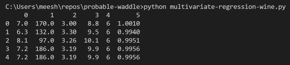
The data looks good to go for the multivariate regression algorithm, so we can start building the model. I do encourage you to try and start with the raw white wine data set to see if you can find a way to get it to the correct format.

Building the model

We need to add a bias term to the data because, as you saw in the explanation of the algorithm, we need it because it's the theta_0 term.

df = pd.concat([pd.Series(1, index=df.index, name='00'), df], axis=1)

Since the data is ready, we can define the independent and dependent variables for the algorithm.

X = df.drop(columns=5)
y = df.iloc[:, 6]

Now let's normalize the data by dividing each column by the max value in that column.

You don't really have to do this step, but it will help speed up the training time for the algorithm. It also helps to prevent one feature from being more dominate than other features.

for i in range(1, len(X.columns)):
	X[i-1] = X[i-1]/np.max(X[i-1])

Let's take a look at the data since the normalization.

print(X.head())

You should see something similar to this in the terminal.

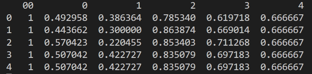
The data is ready now and we can initialize the theta parameter. That just means we're going to make an array of ones that has the same number of columns as the input variable, X.

theta = np.array([1]*len(X.columns))

It should look like this if you print it in your terminal, although you don't need to print it if you don't want to.

[1 1 1 1 1 1]

Then we're going to set the number training points we'll take from the data. We will leave 500 data points out so we can use them for testing later. This is going to be the value for m from the gradient descent equation we went over earlier.

m = len(df) - 500

Now we get to start writing the functions we'll need to train the model after it's built. We'll start with the hypothesis function which is just the input variable multiplied by the theta_n parameter.

def hypothesis(theta, X):
	return theta * X

Next we'll define the cost model which will give us the error margin between the real and predicted values.

def calculateCost(X, y, theta):
    y1 = hypothesis(theta, X)
    y1 = np.sum(y1, axis=1)
    
    return (1 / 2 * m) * sum(np.sqrt((y1 - y) ** 2))

The last function we need before our model is ready to run is a function to calculate gradient descent values.

def gradientDescent(X, y, theta, alpha, i):
    J = [] # cost function for each iteration
    k = 0
    while k < i:
        y1 = hypothesis(theta, X)
        y1 = np.sum(y1, axis=1)
        for c in range(1, len(X.columns)):
            theta[c] = theta[c] - alpha * (1 / m) * (sum((y1 - y) * X.iloc[:, c]))
        j = calculateCost(X, y, theta)
        J.append(j)
        k += 1
    return J, j, theta

With these three functions in place and our data clean, we can finally get to training the model.

Training the model

The training part is the fun part and also the easiest. If you've set your algorithm up correctly, then all you'll have to do is take the optimized parameters it gives you and make predictions.

We're returning a list of costs at each iteration, the final cost, and the optimized theta values from the gradient descent function. So we'll get the optimized theta values and use them for testing.

J, j, theta = gradientDescent(X, y, theta, 0.1, 10000)

After all of the work of setting up the functions and data correctly, this single line of code trains the model and gives us the theta values we need to start predicting values and testing the accuracy of the model.

Testing the model

Now we can test the model by making a prediction using the data.

y_hat = hypothesis(theta, X)
y_hat = np.sum(y_hat, axis=1)

After you’ve checked a few values, you'll know if your model is accurate enough or if you need to do more tuning on the theta values.

If you feel comfortable with your testing results, you can go ahead and start using this model in your projects.

Using the model

The optimized theta values are really all you need to start using the model. You'll continue to use the same equations, even in production, but with the best theta values to give you the most accurate predictions.

You can even continue training the model and try and find better theta values.

Final thoughts

Machine learning has a lot of layers to it, but none of them are too complex. They just start to stack which makes it seem more difficult than it is.

If you're willing to spend some time reading about machine learning libraries and tools, it's really easy to get started. You don't need to know any of the advanced math and statistics to learn the concepts or even to solve real world problems.

The tools are more advanced than they used to be so you can be a machine learning engineer without understanding most of the math behind it.

The main thing you need to understand is how to handle your data. That's the part no one likes to talk about. The algorithms are fun and exciting, but there may be times you need to write SQL procedures to get the raw data you need before you even start processing it.

There are so many applications for machine learning from video games to medicine to manufacturing automation.

Just take some time and make a small model if you're interested in machine learning. As you start to get more comfortable, add on to that model and keep learning more.