
By Milecia McGregor
Most of the tasks machine learning handles right now include things like classifying images, translating languages, handling large amounts of data from sensors, and predicting future values based on current values. You can choose different strategies to fit the problem you're trying to solve.
The good news? There's an algorithm in machine learning that'll handle just about any data you can throw at it. But we'll get there in a minute.
Supervised vs Unsupervised learning
Two of the most commonly used strategies in machine learning include supervised learning and unsupervised learning.
What is supervised learning?
Supervised learning is when you train a machine learning model using labelled data. It means that you have data that already have the right classification associated with them. One common use of supervised learning is to help you predict values for new data.
With supervised learning, you'll need to rebuild your models as you get new data to make sure that the predictions returned are still accurate. An example of supervised learning would be labeling pictures of food. You could have a dataset dedicated to just images of pizza to teach your model what pizza is.
What is unsupervised learning?
Unsupervised learning is when you train a model with unlabeled data. This means that the model will have to find its own features and make predictions based on how it classifies the data.
An example of unsupervised learning would be giving your model pictures of multiple kinds of food with no labels. The dataset would have images of pizza, fries, and other foods and you could use different algorithms to get the model to identify just the images of pizza without any labels.
So what's an algorithm?
When you hear people talk about machine learning algorithms, remember that they are talking about different math equations.
An algorithm is just a customizable math function. That's why most algorithms have things like cost functions, weight values, and parameter functions that you can interchange based on the data you're working with. At its core, machine learning is just a bunch of math equations that need to be solved really fast.
That's why there are so many different algorithms to handle different kinds of data. One particular algorithm is the support vector machine (SVM) and that's what this article is going to cover in detail.
What is an SVM?
Support vector machines are a set of supervised learning methods used for classification, regression, and outliers detection. All of these are common tasks in machine learning.
You can use them to detect cancerous cells based on millions of images or you can use them to predict future driving routes with a well-fitted regression model.
There are specific types of SVMs you can use for particular machine learning problems, like support vector regression (SVR) which is an extension of support vector classification (SVC).
The main thing to keep in mind here is that these are just math equations tuned to give you the most accurate answer possible as quickly as possible.
SVMs are different from other classification algorithms because of the way they choose the decision boundary that maximizes the distance from the nearest data points of all the classes. The decision boundary created by SVMs is called the maximum margin classifier or the maximum margin hyper plane.
How an SVM works
A simple linear SVM classifier works by making a straight line between two classes. That means all of the data points on one side of the line will represent a category and the data points on the other side of the line will be put into a different category. This means there can be an infinite number of lines to choose from.
What makes the linear SVM algorithm better than some of the other algorithms, like k-nearest neighbors, is that it chooses the best line to classify your data points. It chooses the line that separates the data and is the furthest away from the closet data points as possible.
A 2-D example helps to make sense of all the machine learning jargon. Basically you have some data points on a grid. You're trying to separate these data points by the category they should fit in, but you don't want to have any data in the wrong category. That means you're trying to find the line between the two closest points that keeps the other data points separated.
So the two closest data points give you the support vectors you'll use to find that line. That line is called the decision boundary.
 Linear SVM
The decision boundary doesn't have to be a line. It's also referred to as a hyperplane because you can find the decision boundary with any number of features, not just two.
 Non-linear SVM using RBF kernel
Types of SVMs
There are two different types of SVMs, each used for different things:
- Simple SVM: Typically used for linear regression and classification problems.
- Kernel SVM: Has more flexibility for non-linear data because you can add more features to fit a hyperplane instead of a two-dimensional space.
Why SVMs are used in machine learning
SVMs are used in applications like handwriting recognition, intrusion detection, face detection, email classification, gene classification, and in web pages. This is one of the reasons we use SVMs in machine learning. It can handle both classification and regression on linear and non-linear data.
Another reason we use SVMs is because they can find complex relationships between your data without you needing to do a lot of transformations on your own. It's a great option when you are working with smaller datasets that have tens to hundreds of thousands of features. They typically find more accurate results when compared to other algorithms because of their ability to handle small, complex datasets.
Here are some of the pros and cons for using SVMs.
Pros
- Effective on datasets with multiple features, like financial or medical data.
- Effective in cases where number of features is greater than the number of data points.
- Uses a subset of training points in the decision function called support vectors which makes it memory efficient.
- Different kernel functions can be specified for the decision function. You can use common kernels, but it's also possible to specify custom kernels.
Cons
- If the number of features is a lot bigger than the number of data points, avoiding over-fitting when choosing kernel functions and regularization term is crucial.
- SVMs don't directly provide probability estimates. Those are calculated using an expensive five-fold cross-validation.
- Works best on small sample sets because of its high training time.
Since SVMs can use any number of kernels, it's important that you know about a few of them.
Kernel functions
Linear
These are commonly recommended for text classification because most of these types of classification problems are linearly separable.
The linear kernel works really well when there are a lot of features, and text classification problems have a lot of features. Linear kernel functions are faster than most of the others and you have fewer parameters to optimize.
Here's the function that defines the linear kernel:
f(X) = w^T * X + b
In this equation, w is the weight vector that you want to minimize, X is the data that you're trying to classify, and b is the linear coefficient estimated from the training data. This equation defines the decision boundary that the SVM returns.
Polynomial
The polynomial kernel isn't used in practice very often because it isn't as computationally efficient as other kernels and its predictions aren't as accurate.
Here's the function for a polynomial kernel:
f(X1, X2) = (a + X1^T * X2) ^ b
This is one of the more simple polynomial kernel equations you can use. f(X1, X2) represents the polynomial decision boundary that will separate your data. X1 and X2 represent your data.
Gaussian Radial Basis Function (RBF)
One of the most powerful and commonly used kernels in SVMs. Usually the choice for non-linear data.
Here's the equation for an RBF kernel:
f(X1, X2) = exp(-gamma * ||X1 - X2||^2)
In this equation, gamma specifies how much a single training point has on the other data points around it. ||X1 - X2|| is the dot product between your features.
Sigmoid
More useful in neural networks than in support vector machines, but there are occasional specific use cases.
Here's the function for a sigmoid kernel:
f(X, y) = tanh(alpha * X^T * y + C)
In this function, alpha is a weight vector and C is an offset value to account for some mis-classification of data that can happen.
Others
There are plenty of other kernels you can use for your project. This might be a decision to make when you need to meet certain error constraints, you want to try and speed up the training time, or you want to super tune parameters.
Some other kernels include: ANOVA radial basis, hyperbolic tangent, and Laplace RBF.
Now that you know a bit about how the kernels work under the hood, let's go through a couple of examples.
Examples with datasets
To show you how SVMs work in practice, we'll go through the process of training a model with it using the Python Scikit-learn library. This is commonly used on all kinds of machine learning problems and works well with other Python libraries.
Here are the steps regularly found in machine learning projects:
- Import the dataset
- Explore the data to figure out what they look like
- Pre-process the data
- Split the data into attributes and labels
- Divide the data into training and testing sets
- Train the SVM algorithm
- Make some predictions
- Evaluate the results of the algorithm
Some of these steps can be combined depending on how you handle your data. We'll do an example with a linear SVM and a non-linear SVM. You can find the code for these examples here.
Linear SVM Example
We'll start by importing a few libraries that will make it easy to work with most machine learning projects.
import matplotlib.pyplot as plt
import numpy as np
from sklearn import svm
For a simple linear example, we'll just make some dummy data and that will act in the place of importing a dataset.
# linear data
X = np.array([1, 5, 1.5, 8, 1, 9, 7, 8.7, 2.3, 5.5, 7.7, 6.1])
y = np.array([2, 8, 1.8, 8, 0.6, 11, 10, 9.4, 4, 3, 8.8, 7.5])
The reason we're working with numpy arrays is to make the matrix operations faster because they use less memory than Python lists. You could also take advantage of typing the contents of the arrays. Now let's take a look at what the data look like in a plot:
# show unclassified data
plt.scatter(X, y)
plt.show()
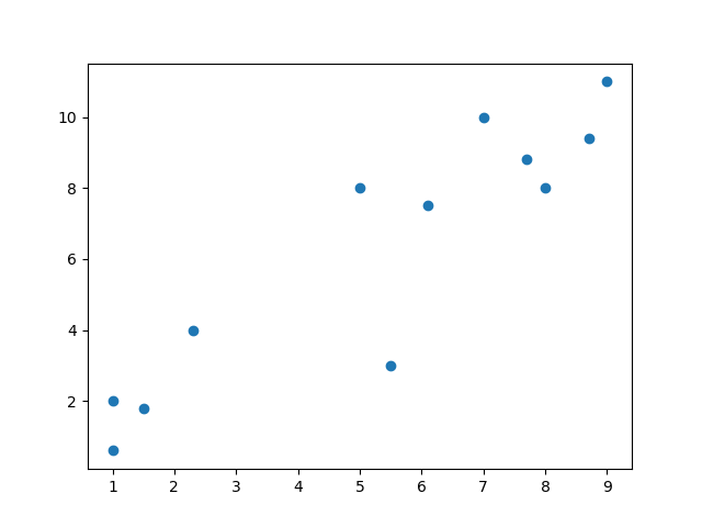
Once you see what the data look like, you can take a better guess at which algorithm will work best for you. Keep in mind that this is a really simple dataset, so most of the time you'll need to do some work on your data to get it to a usable state.
We'll do a bit of pre-processing on the already structured code. This will put the raw data into a format that we can use to train the SVM model.
# shaping data for training the model
training_X = np.vstack((X, y)).T
training_y = [0, 1, 0, 1, 0, 1, 1, 1, 0, 0, 1, 1]
Now we can create the SVM model using a linear kernel.
# define the model
clf = svm.SVC(kernel='linear', C=1.0)
That one line of code just created an entire machine learning model. Now we just have to train it with the data we pre-processed.
# train the model
clf.fit(training_X, training_y)
That's how you can build a model for any machine learning project. The dataset we have might be small, but if you encounter a real-world dataset that can be classified with a linear boundary this model still works.
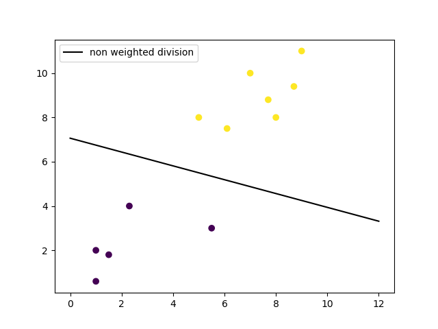
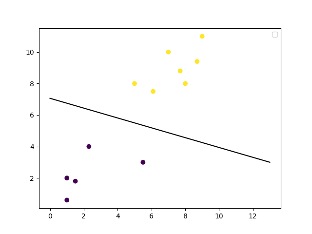
With your model trained, you can make predictions on how a new data point will be classified and you can make a plot of the decision boundary. Let's plot the decision boundary.
# get the weight values for the linear equation from the trained SVM model
w = clf.coef_[0]

# get the y-offset for the linear equation
a = -w[0] / w[1]

# make the x-axis space for the data points
XX = np.linspace(0, 13)

# get the y-values to plot the decision boundary
yy = a * XX - clf.intercept_[0] / w[1]

# plot the decision boundary
plt.plot(XX, yy, 'k-')

# show the plot visually
plt.scatter(training_X[:, 0], training_X[:, 1], c=training_y)
plt.legend()
plt.show()
Non-Linear SVM Example
For this example, we'll use a slightly more complicated dataset to show one of the areas SVMs shine in. Let's import some packages.
import matplotlib.pyplot as plt
import numpy as np
from sklearn import datasets
from sklearn import svm
This set of imports is similar to those in the linear example, except it imports one more thing. Now we can use a dataset directly from the Scikit-learn library.
# non-linear data
circle_X, circle_y = datasets.make_circles(n_samples=300, noise=0.05)
The next step is to take a look at what this raw data looks like with a plot.
# show raw non-linear data
plt.scatter(circle_X[:, 0], circle_X[:, 1], c=circle_y, marker='.')
plt.show()
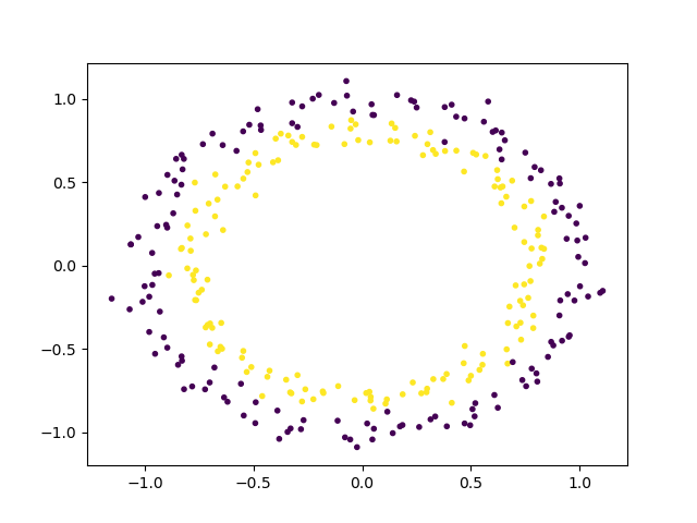
Now that you can see how the data are separated, we can choose a non-linear SVM to start with. This dataset doesn't need any pre-processing before we use it to train the model, so we can skip that step. Here's how the SVM model will look for this:
# make non-linear algorithm for model
nonlinear_clf = svm.SVC(kernel='rbf', C=1.0)
In this case, we'll go with an RBF (Gaussian Radial Basis Function) kernel to classify this data. You could also try the polynomial kernel to see the difference between the results you get. Now it's time to train the model.
# training non-linear model
nonlinear_clf.fit(circle_X, circle_y)
You can start labeling new data in the correct category based on this model. To see what the decision boundary looks like, we'll have to make a custom function to plot it.
# Plot the decision boundary for a non-linear SVM problem
def plot_decision_boundary(model, ax=None):
    if ax is None:
        ax = plt.gca()

    xlim = ax.get_xlim()
    ylim = ax.get_ylim()

    # create grid to evaluate model
    x = np.linspace(xlim[0], xlim[1], 30)
    y = np.linspace(ylim[0], ylim[1], 30)
    Y, X = np.meshgrid(y, x)

    # shape data
    xy = np.vstack([X.ravel(), Y.ravel()]).T

    # get the decision boundary based on the model
    P = model.decision_function(xy).reshape(X.shape)

    # plot decision boundary
    ax.contour(X, Y, P,
               levels=[0], alpha=0.5,
               linestyles=['-'])
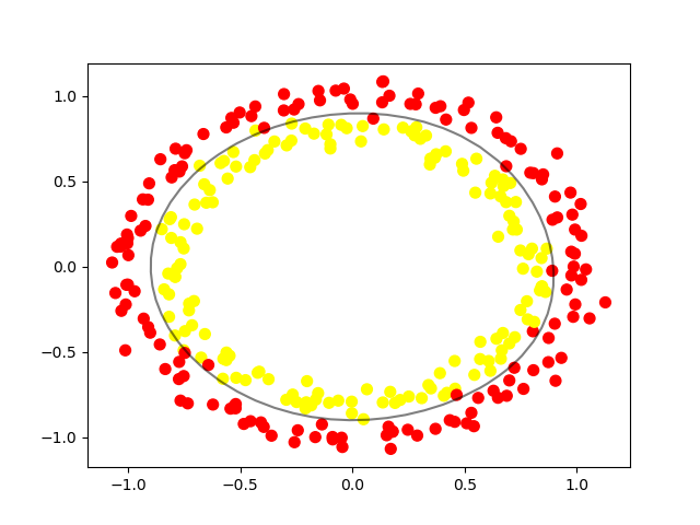
You have everything you need to plot the decision boundary for this non-linear data. We can do that with a few lines of code that use the Matlibplot library, just like the other plots.
# plot data and decision boundary
plt.scatter(circle_X[:, 0], circle_X[:, 1], c=circle_y, s=50)
plot_decision_boundary(nonlinear_clf)
plt.scatter(nonlinear_clf.support_vectors_[:, 0], nonlinear_clf.support_vectors_[:, 1], s=50, lw=1, facecolors='none')
plt.show()
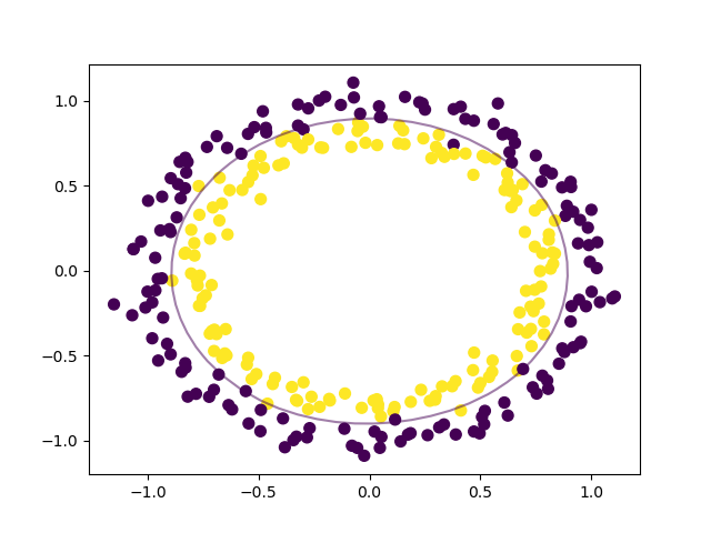
When you have your data and you know the problem you're trying to solve, it really can be this simple.
You can change your training model completely, you can choose different algorithms and features to work with, and you can fine tune your results based on multiple parameters. There are libraries and packages for all of this now so there's not a lot of math you have to deal with.
Tips for real world problems
Real world datasets have some common issues because of how large they can be, the varying data types they hold, and how much computing power they can need to train a model.
There are a few things you should watch out for with SVMs in particular:
- Make sure that your data are in numeric form instead of categorical form. SVMs expect numbers instead of other kinds of labels.
- Avoid copying data as much as possible. Some Python libraries will make duplicates of your data if they aren't in a specific format. Copying data will also slow down your training time and skew the way your model assigns the weights to a specific feature.
- Watch your kernel cache size because it uses your RAM. If you have a really large dataset, this could cause problems for your system.
- Scale your data because SVM algorithms aren't scale invariant. That means you can convert all of your data to be within the ranges of [0, 1] or [-1, 1].
Other thoughts
You might wonder why I didn't go into the deep details of the math here. It's mainly because I don't want to scare people away from learning more about machine learning.
It's fun to learn about those long, complicated math equations and their derivations, but it's rare you'll be writing your own algorithms and writing proofs on real projects.
It's like using most of the other stuff you do every day, like your phone or your computer. You can do everything you need to do without knowing the how the processors are built.
Machine learning is like any other software engineering application. There are a ton of packages that make it easier for you to get the results you need without a deep background in statistics.
Once you get some practice with the different packages and libraries available, you'll find out that the hardest part about machine learning is getting and labeling your data.
I'm working on a neuroscience, machine learning, web-based thing! You should follow me on Twitter to learn more about it and other cool tech stuff.