
By Moshe Binieli
Introduction
This article will deal with the statistical method mean squared error, and I’ll describe the relationship of this method to the regression line.
The example consists of points on the Cartesian axis. We will define a mathematical function that will give us the straight line that passes best between all points on the Cartesian axis.
And in this way, we will learn the connection between these two methods, and how the result of their connection looks together.
General explanation
This is the definition from Wikipedia:
In statistics, the mean squared error (MSE) of an estimator (of a procedure for estimating an unobserved quantity) measures the average of the squares of the errors — that is, the average squared difference between the estimated values and what is estimated. MSE is a risk function, corresponding to the expected value of the squared error loss. The fact that MSE is almost always strictly positive (and not zero) is because of randomness or because the estimator does not account for information that could produce a more accurate estimate.
The structure of the article
- Get a feel for the idea, graph visualization, mean squared error equation.
- The mathematical part which contains algebraic manipulations and a derivative of two-variable functions for finding a minimum. This section is for those who want to understand how we get the mathematical formulas later, you can skip it if that doesn’t interest you.
- An explanation of the mathematical formulae we received and the role of each variable in the formula.
- Examples
Get a feel for the idea
Let’s say we have seven points, and our goal is to find a line that minimizes the squared distances to these different points.
Let’s try to understand that.
I will take an example and I will draw a line between the points. Of course, my drawing isn’t the best, but it’s just for demonstration purposes.
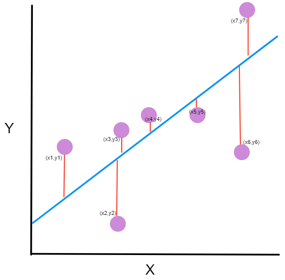
You might be asking yourself, what is this graph?
- the purple dots are the points on the graph. Each point has an x-coordinate and a y-coordinate.
- The blue line is our prediction line. This is a line that passes through all the points and fits them in the best way. This line contains the predicted points.
- The red line between each purple point and the prediction line are the errors. Each error is the distance from the point to its predicted point.
You should remember this equation from your school days, y=Mx+B, where M is the slope of the line and B is y-intercept of the line.
We want to find M (slope) and B (y-intercept) that minimizes the squared error!
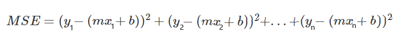
Let’s define a mathematical equation that will give us the mean squared error for all our points.
Let’s analyze what this equation actually means.
- In mathematics, the character that looks like weird E is called summation (Greek sigma). It is the sum of a sequence of numbers, from i=1 to n. Let’s imagine this like an array of points, where we go through all the points, from the first (i=1) to the last (i=n).
- For each point, we take the y-coordinate of the point, and the y’-coordinate. The y-coordinate is our purple dot. The y’ point sits on the line we created. We subtract the y-coordinate value from the y’-coordinate value, and calculate the square of the result.
- The third part is to take the sum of all the (y-y’)² values, and divide it by n, which will give the mean.
Our goal is to minimize this mean, which will provide us with the best line that goes through all the points.
From concept to mathematical equations
This part is for people who want to understand how we got to the mathematical equations. You can skip to the next part if you want.
As you know, the line equation is y=mx+b, where m is the slope and b is the y-intercept.
Let’s take each point on the graph, and we’ll do our calculation (y-y’)².
But what is y’, and how do we calculate it? We do not have it as part of the data.
But we do know that, in order to calculate y’, we need to use our line equation, y=mx+b, and put the x in the equation.
From here we get the following equation:
Let’s rewrite this expression to simplify it.

Let’s begin by opening all the brackets in the equation. I colored the difference between the equations to make it easier to understand.
Now, let’s apply another manipulation. We will take each part and put it together. We will take all the y, and (-2ymx) and etc, and we will put them all side-by-side.
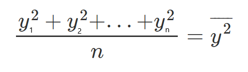
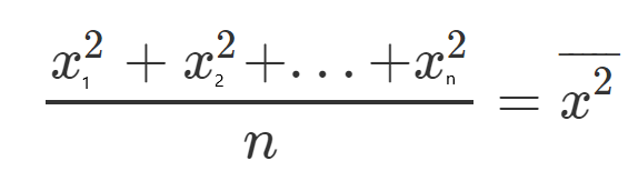
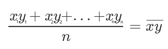
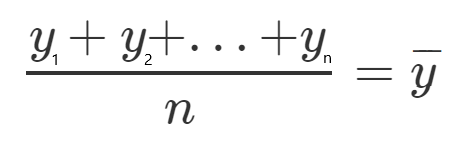
At this point we’re starting to be messy, so let’s take the mean of all squared values for y, xy, x, x².
Let’s define, for each one, a new character which will represent the mean of all the squared values.
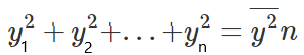
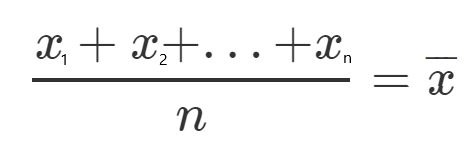
Let’s see an example, let’s take all the y values, and divide them by n since it’s the mean, and call it y(HeadLine).
If we multiply both sides of the equation by n we get:
Which will lead us to the following equation:

If we look at what we got, we can see that we have a 3D surface. It looks like a glass, which rises sharply upwards.
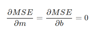
We want to find M and B that minimize the function. We will make a partial derivative with respect to M and a partial derivative with respect to B.
Since we are looking for a minimum point, we will take the partial derivatives and compare to 0.
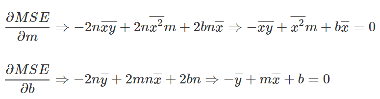
Let’s take the two equations we received, isolating the variable b from both, and then subtracting the upper equation from the bottom equation.
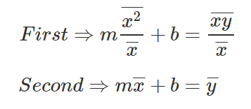
Let’s subtract the first equation from the second equation
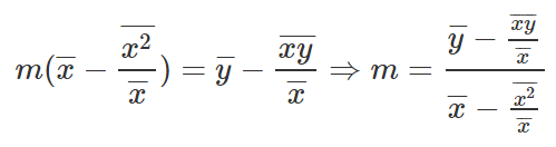
Let’s get rid of the denominators from the equation.
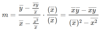
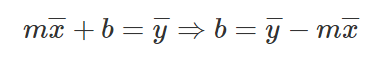
And there we go, this is the equation to find M, let’s take this and write down B equation.
Equations for slope and y-intercept
Let’s provide the mathematical equations that will help us find the required slope and y-intercept.
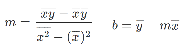
So you probably thinking to yourself, what the heck are those weird equations?
They are actually simple to understand, so let’s talk about them a little bit.
Now that we understand our equations it’s time to get all things together and show some examples.
Examples
A big thank you to Khan Academy for the examples.
Example #1
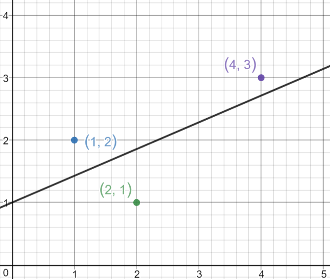
Let’s take 3 points, (1,2), (2,1), (4,3).

Let’s find M and B for the equation y=mx+b.
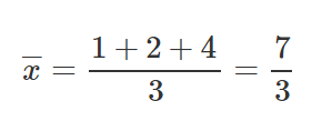
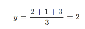
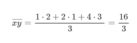
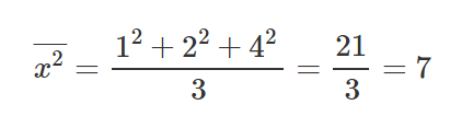
After we’ve calculated the relevant parts for our M equation and B equation, let’s put those values inside the equations and get the slope and y-intercept.
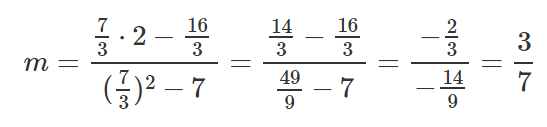

Let’s take those results and set them inside the line equation y=mx+b.

Now let’s draw the line and see how the line passes through the lines in such a way that it minimizes the squared distances.
Example #2
Let’s take 4 points, (-2,-3), (-1,-1), (1,2), (4,3).

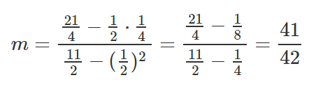
Let’s find M and B for the equation y=mx+b.
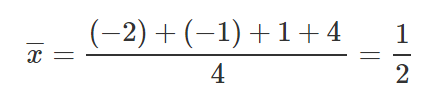

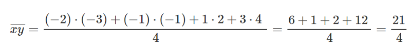

Same as before, let’s put those values inside our equations to find M and B.

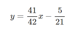
Let’s take those results and set them inside line equation y=mx+b.
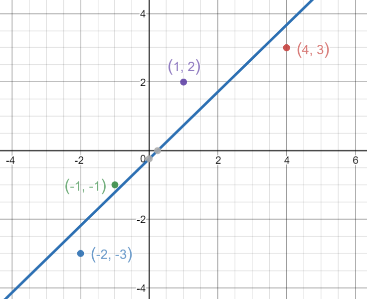
Now let’s draw the line and see how the line passes through the lines in such a way that it minimizes the squared distances.
In conclusion
As you can see, the whole idea is simple. We just need to understand the main parts and how we work with them.
You can work with the formulas to find the line on another graph, and perform a simple calculation and get the results for the slope and y-intercept.
That’s all, simple eh? ?
Every comment and all feedback is welcome — if it’s necessary, I will fix the article.
Feel free to contact me directly at LinkedIn — Click Here.