Machine Learning in Python – The Top New Scikit-Learn 0.24 Features You Should Know

Scikit-learn is one of the most popular open-source and free machine learning libraries for Python.

The scikit-learn library contains a lot of efficient tools for machine learning and statistical modeling including classification, regression, clustering, and dimensionality reduction.

Many data scientists, machine learning engineers, and researchers rely on this library for their machine learning projects. I personally love using the scikit-learn library because it offers a ton of flexibility and it’s easy to understand its documentation with a lot of examples.

In this article, I’m happy to share with you the five best new features in scikit-learn 0.24.

First, Install the Latest Version of the Scikit-Learn Library

Firstly, make sure you install the latest version (with pip):

pip install --upgrade scikit-learn

If you are using conda, use the following command:

conda install -c conda-forge scikit-learn

Note: This version supports Python versions 3.6 to 3.9.

Now, let’s look at the new features!

Mean Absolute Percentage Error (MAPE)

The new version of scikit-learn introduces a new evaluation metric for a regression problem called Mean Absolute Percentage Error(MAPE). Previously you could calculate MAPE by using a piece of code.

np.mean(np.abs((y_test — preds)/y_test))

But now you can call a function called mean_absolute_percentage_error from the sklearn.metrics module to evaluate the performance of your regression model.

Example:

from sklearn.metrics import mean_absolute_percentage_error
y_true = [3, -0.5, 2, 7]
y_pred = [2.5, 0.0, 2, 8]

print(mean_absolute_percentage_error(y_true, y_pred))

0.3273809523809524

Note: Keep in mind that the function does not represent the output as a percentage in the range [0, 100]. Instead, we represent it in the range [0, 1/eps]. The best value is 0.0.

OneHotEncoder Supports Missing Values

OneHotEncoder can now handle missing values if presented in the dataset. It treats a missing value as a category. Let’s understand more about how it works in the following example.

First import the important packages:

import pandas as pd 
import numpy as np
from sklearn.preprocessing import OneHotEncoder

Create a simple data-frame with a categorical feature that has missing values:

# intialise data of lists.
data = {'education_level':['primary', 'secondary', 'bachelor', np.nan,'masters',np.nan]}
  
# Create DataFrame
df = pd.DataFrame(data)
  
# Print the output.
print(df)

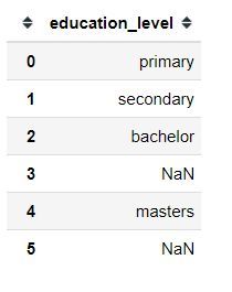
As you can see, we have two missing values in our education_level column.

Create the instance of OneHotEncoder:

enc = OneHotEncoder()

Then fit and transform our data:

enc.fit_transform(df).toarray()

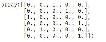
Our education_level column has been transformed and all missing values treated as a new category (check the last column of the above array).

New Method for Feature Selection

SequentialFeatureSelector is a new method for feature selection in scikit-learn. It can be either forward selection or backward selection.

Forward Selection

Forward Selection iteratively finds the best new feature and then adds it to the set of selected features.

This means we start with zero features and then find a feature that maximizes the cross-validation score of an estimator. The selected feature is added to the set and the procedure is repeated until we reach our desired number of selected features.

Backward Selection

This second selection follows the same idea but in a different direction. Here we start with all features and then remove a feature from the set until we reach the desired number of selected features.

Example

Import the important packages:

from sklearn.feature_selection import SequentialFeatureSelector
from sklearn.neighbors import KNeighborsClassifier
from sklearn.datasets import load_iris

Load the iris dataset and its feature names:

X, y = load_iris(return_X_y=True, as_frame=True)
feature_names = X.columns

Create the instance of the estimator:

knn = KNeighborsClassifier(n_neighbors=3)

Create the instance of SequentialFeatureSelector, set the number of features to select to be 2, and set the direction to be “backward”:

sfs = SequentialFeatureSelector(knn, n_features_to_select=2,direction='backward')

Finally learn the features to select:

sfs.fit(X,y)

Show selected features:

print("Features selected by backward sequential selection: "f{feature_names[sfs.get_support()].tolist()}")

Features selected by backward sequential selection: [‘petal length (cm)’, ‘petal width (cm)’].

The only downside of this new feature selection method is that it can be slower than other methods you already know (SelectFromModel & RFE ) because it evaluates models with cross-validation.

New Methods for Hyper-Parameter Tuning

When it comes to hyper-parameter tuning, GridSearchCV and RandomizedSearchCv from Scikit-learn have been the first choice for many data scientists.

But in the new version, we have two new classes for hyper-parameter tuning called HalvingGridSearchCV and HalvingRandomSearchCV.

HalvingGridSearchCV and HalvingRandomSearchCV use a new approach called successive halving to find the best hyperparameters. Successive halving is like competition or tournament among all hyperparameter combinations.

How does successive halving work?

In the first iteration, they train a combination of hyper-parameters on a subset of observations (training data).

Then in the next iteration, it selects only a combination of hyper-parameters that have good performance in the first iteration and they will be trained in a large number of observations to compete.

So it repeats this selection process in each iteration until it selects the best combination of hyperparameters in the final iteration.

Note: These classes are still experimental:

Example:

Import the important packages:

from sklearn.datasets import make_classification
from sklearn.ensemble import RandomForestClassifier
from sklearn.experimental import enable_halving_search_cv  
from sklearn.model_selection import HalvingRandomSearchCV
from scipy.stats import randint

Since these new classes are still experimental, to use them, we explicitly import enable_halving_search_cv.

Create a classification dataset by using the make_classification method:

X, y = make_classification(n_samples=1000)

Create the instance of the estimator. Here we use a Random Forest Classifier:

clf = RandomForestClassifier(n_estimators=20)

Create parameter distribution for tuning:

param_dist = {"max_depth": [3, None],
              "max_features": randint(1, 11),
              "min_samples_split": randint(2, 11),
              "bootstrap": [True, False],
              "criterion": ["gini", "entropy"]}

Then we instantiate the HalvingGridSearchCV class with the RandomForestClassifier as an estimator and the list of parameter distributions:

rsh = HalvingRandomSearchCV(
    estimator=clf,
    param_distributions=param_dist,
    cv = 5,
    factor=2,
    min_resources = 20)

There are two important parameters in HalvingRandomSearchCV you need to know.

1. factor — This determines the proportion of the combination of hyper-parameters that are selected for each subsequent iteration. For example, factor=3 means that only one-third of the candidates are selected for the next iteration.
2. min_resources is the amount of resources (number of observations) allocated at the first iteration for each combination of hyper-parameters.

Finally, we can fit the search object that we have created with our dataset.

rsh.fit(X,y)

After training, we can see different output such as:

The number of iterations

print(rsh.n_iterations_ )

which is 6.

Or the number of candidate parameters that were evaluated at each iteration

print(rsh.n_candidates_ )

which is [50, 25, 13, 7, 4, 2].

Or the number of resources used at each iteration:

print(rsh.n_resources_)

which is [20, 40, 80, 160, 320, 640].

Or parameter setting that gave the best results on the hold-out data:

print(rsh.best_params_)

{‘bootstrap’: False,
‘criterion’: ‘entropy’,
‘max_depth’: None,
‘max_features’: 5,
‘min_samples_split’: 2}

New self-training meta-estimator for semi-supervised learning

Scikit-learn 0.24 has introduced a new self-training implementation for semi-supervised learning called SelfTrainingclassifier. You can use SelfTrainingClassifier with any supervised classifier that can return probability estimates for each class.

This means any supervised classifier can function as a semi-supervised classifier, allowing it to learn from unlabeled observations in the dataset.

Note: The unlabeled values in the target column must have a value of -1.

Let’s understand more about how it works in the following example.

Import the important packages:

import numpy as np
from sklearn import datasets
from sklearn.semi_supervised import SelfTrainingClassifier
from sklearn.svm import SVC

In this example, we will use the iris dataset and the Super vector machine algorithm as a supervised classifier (it can implement fit and predict_proba).

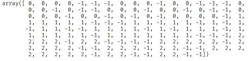
Then we load the dataset and select randomly some of the observations to be unlabeled:

rng = np.random.RandomState(42)
iris = datasets.load_iris()
random_unlabeled_points = rng.rand(iris.target.shape[0]) < 0.3
iris.target[random_unlabeled_points] = -1

As you can see, unlabeled values in the target column have a value of -1.

Create an instance of the supervised estimator:

svc = SVC(probability=True, gamma="auto")

Create an instance of the self-training meta estimator and add svc as a base_estimator:

self_training_model = SelfTrainingClassifier(base_estimator=svc)

Finally, we can train self_traning_model on the iris dataset that has some unlabeled observations:

self_training_model.fit(iris.data, iris.target)

SelfTrainingClassifier(base_estimator=SVC(gamma=’auto’, probability=True))

Final Thoughts on Scikit-Learn 0.24

As I said, scikit-learn remains one the most popular open-source machine learning libraries. And it has all the features you need to build an end-to-end machine learning project.

You can also implement the new impressive features presented in this article in your machine learning project.

You can find the highlights of other features released in scikit-learn 0.24 here.

Congratulations 👏👏, you have made it to the end of this article! I hope you have learned something new that will help you on your next machine learning or data science project.

If you learned something new or enjoyed reading this article, please share it so that others can see it. Until then, see you in the next post!

You can also find me on Twitter @Davis_McDavid.

You can read other articles here.