
By Yacine Mahdid
In this tutorial we'll learn how to automatically publish machine learning models in a Gitlab package registry and make them available for your teammates to use. You can also use this technique to share a packaged version of your code as a binary.
If you are a beginner Gitlab user and are unfamiliar with CI/CD techniques, this tutorial is for you! A basic understanding of how machine-learning and deep learning is a plus, but it isn't a requirement to understand the CI/CD publishing part.
Here's what we'll cover:
- Gitlab Code Setup
- Deep Convolutional Neural Network Code
- Image Recognition Code
- Branching Methodology
- CI/CD Uploading
- Conclusion
First, Some Background
At some point during your machine learning engineer career you might need to share a model you've trained with other developers. There are multiple ways of doing this.
Give access to the repository
If you don't mind showing your whole code, this is a very viable option.
If you use a good branching methodology your colleagues will only need to look at the main branch in order to figure out what's the most up to date model they can use. Then they can check the README.md to learn how to use it.
However, giving full access to the repository might not be a viable option for you.
Share the latest model manually
Another way would be to extract the relevant code that you want to make public and send it to them manually.
This can become a bit of a mess if you are working with more than one person because the model you send might not be up to date. It also puts the burden on you to make sure that people are always using the latest version of your model.
Share the latest model automatically
A simpler solution, even in the case where the repository code is available, is to put the packaging burden on a CI/CD pipeline.
This is the topic of this tutorial, and our setup will look like this:
- The code repository, CI/CD tool set, and package registry will be on Gitlab
- The code we'll be packaging will be a simple trained PyTorch neural network on the MNIST dataset for digit recognition.
- All the instructions and the requirements will be available in the package.
🚨 Disclaimer 🚨: This isn't how you should deploy a PyTorch production-ready model! To learn how to do this, check out this tutorial on TorchScript.
Let's get started.
Gitlab Code Setup
For this tutorial we will bundle four files:
- model.pth: which is a pickled version of the latest version of the trained model.
- run_mnist.py: simple Python script to run the model to detect a digit from a png image.
- requirements.txt: text file containing all the dependencies required to run the model.
- INSTRUCTION.md: step by step instructions to use the package.
The package can then be used freely by anyone who has access to the package registry and will be automatically updated.
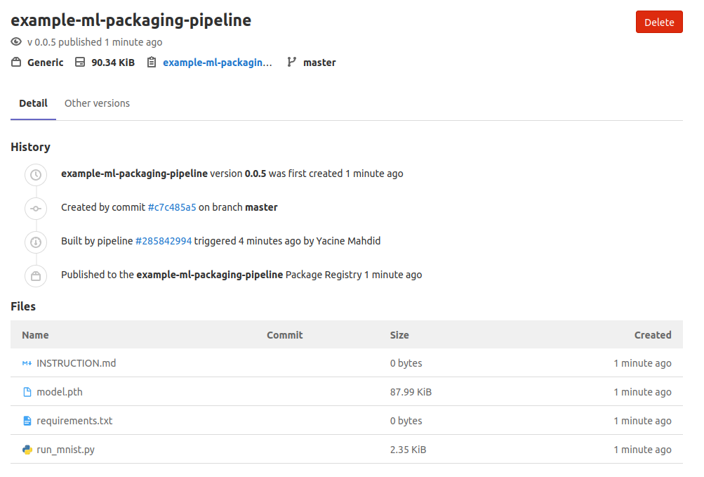 The package will then look like this on Gitlab Package Registry!
Let's jump into the neural network code, which is a modified version of this comprehensive article on digit recognition. The modified code can be found over at my public Gitlab repository.
Deep Convolutional Neural Network Code
In the section below, you will see quite a lot of terminology about deep neural networks. This isn't a tutorial on neural networks, so if you feel a bit overwhelmed by the specifics you can jump directly to the Branching Methodology section.
Just keep in mind that we've trained some sort of image recognition program that, given a .png file representing a digit, will be able to tell you what number it contains.
However, for those that want to get a better understanding about how Deep Neural Networks work under the hood, you can take a look at my tutorial where I build one from scratch or checkout the code directly in my Github.
Neural Network Definition
The network definition code is very straightforward since the network we will use is simple. It has the following characteristics:
- 2 convolutional layers.
- Dropout is applied on the second convolutional layer.
- Relu activation functions applied on all neurons.
- 2 fully connected layers at the end for inference.
import torch
import torchvision

import torch.nn as nn
import torch.nn.functional as F
import torch.optim as optim


# Define the network
# It's a 2 convolutional layer with dropout at the 2nd and finally 2 fully connected layer
# All layers use relu
class Net(nn.Module):
    def __init__(self):
        super(Net, self).__init__()
        self.conv1 = nn.Conv2d(1, 10, kernel_size=5)
        self.conv2 = nn.Conv2d(10, 20, kernel_size=5)
        self.conv2_drop = nn.Dropout2d()
        self.fc1 = nn.Linear(320, 50)
        self.fc2 = nn.Linear(50, 10)

    def forward(self, x):
        x = F.relu(F.max_pool2d(self.conv1(x), 2))
        x = F.relu(F.max_pool2d(self.conv2_drop(self.conv2(x)), 2))
        x = x.view(-1, 320)
        x = F.relu(self.fc1(x))
        x = F.dropout(x, training=self.training)
        x = self.fc2(x)
        return F.log_softmax(x, dim=1)
Training Function
We then created a utility training function in order to iteratively improve our defined network using gradient descent. If you want to learn more about how gradient descent works check out my short tutorial on it.
This training regimen will do the following:
- Iterate on batches of training data representing 28 by 28 digits.
- Use the negative log likelihood cost function to calculate the loss.
- Calculate gradients.
- Optimize the weights of the network using gradient descent.
- Save the model at fixed intervals.
def train(network, optimizer, train_loader, epoch_id, log_interval=10):
  """Run the training regiment on the training set using train_loader

    Args:
        network: The instantiated network.
        optimizer: The optimizer used to change the weights.
        train_loader: the loader for the training set already setup
        epoch_id: the current id of the epoch used for cosmetic reason.
        log_interval: interval at which we print an output

    Returns:
        nothing, will save directly at root level the model and the optimizer state

  """

  # Set the network in training mode
  network.train()

  # Iterate over the full training set
  for batch_idx, (data, target) in enumerate(train_loader):

    # Calculate the gradients for this batch of data
    optimizer.zero_grad()
    output = network(data)
    loss = F.nll_loss(output, target)
    loss.backward()

    # Optimize the network
    optimizer.step()

    # Log and save every selected interval
    if batch_idx % log_interval == 0:

      print('Train Epoch: {} [{}/{} ({:.0f}%)]\tLoss: {:.6f}'.format(
        epoch_id, batch_idx * len(data), len(train_loader.dataset),
        100. * batch_idx / len(train_loader), loss.item()))

      # This will save the state as a pickled object
      torch.save(network.state_dict(), './model.pth')
      torch.save(optimizer.state_dict(), './optimizer.pth')
The data for training can be found over here on the Yan LeCun website. Here we are using the datasets formatted as 28 by 28 PyTorch tensors for training.
Testing Function
The next function we create is a testing function to validate if our network has learned something without reusing the same training data. This function is simple in the sense that it will just tally the correct and incorrect predictions.
def test(network, test_loader):
  """Run the testing regiment on the test set using test_loader

    Args:
        network: The instantiated and trained network.
        test_loader: the loader for the testing set already setup

    Returns:
        nothing, will only print result

  """

  # Variable instantiation
  test_loss = 0
  correct = 0

  # Move the network to evaluate mode instead of training
  network.eval()

  # setup torch so to not track any  gradient
  with torch.no_grad():

    # Iterate on all the test data and accumulate the loss
    for data, target in test_loader:
      output = network(data)
      test_loss += F.nll_loss(output, target, size_average=False).item()
      pred = output.data.max(1, keepdim=True)[1]
      correct += pred.eq(target.data.view_as(pred)).sum()

  # Average loss calculation and printing
  test_loss /= len(test_loader.dataset)
  print('\nTest set: Avg. loss: {:.4f}, Accuracy: {}/{} ({:.0f}%)\n'.format(
    test_loss, correct, len(test_loader.dataset),
    100. * correct / len(test_loader.dataset)))
This function will be useful to check how well our network has learned after each training iteration.
Training Regimen
Finally, we can tie all of the above together with the main body of the training script! A few things are happening, but the most important points are the following:
- We set our hyper parameters statically. A better way to define them would be to use a validation set to figure them out based on the data.
- We create our data loader which will ingest data and spit out tensors in the right shape for the network. These loader will transform the data by normalizing them with the global mean and standard deviation for the MNIST datasets.
- We use stochastic gradient descent with momentum as the optimization method, which is one of the many flavors of gradient descent we can use.
- We loop through the full training dataset's "epoch", the amount of time to train the network while testing on the held-out test datasets.
# Experimental Parameters that we can tweak
n_epochs = 3
batch_size_train = 64
batch_size_test = 1000
learning_rate = 0.01
momentum = 0.5

# Variable from the dataset that should stay as is
global_mean_mnist = 0.1307
global_std_mnist = 0.3081


# Random Seed for Reproducible Experimentation
random_seed = 42
torch.backends.cudnn.enabled = False
torch.manual_seed(random_seed)


# Data Loader to gather the data and then normalize them
train_loader = torch.utils.data.DataLoader(
  torchvision.datasets.MNIST('./data/', train=True, download=True,
                             transform=torchvision.transforms.Compose([
                               torchvision.transforms.ToTensor(),
                               torchvision.transforms.Normalize(
                                 (global_mean_mnist,), (global_std_mnist,))
                             ])),
  batch_size=batch_size_train, shuffle=True)

test_loader = torch.utils.data.DataLoader(
  torchvision.datasets.MNIST('./data/', train=False, download=True,
                             transform=torchvision.transforms.Compose([
                               torchvision.transforms.ToTensor(),
                               torchvision.transforms.Normalize(
                                 (global_mean_mnist,), (global_std_mnist,))
                             ])),
  batch_size=batch_size_test, shuffle=True)

# Initialize network and optimizer
network = Net()
optimizer = optim.SGD(network.parameters(), lr=learning_rate,
                      momentum=momentum)

# Test first to show that the model didn't learn a thing
test(network, test_loader)

# Train on the whole dataset multiple time and test
for epoch_id in range(1, n_epochs + 1):
  train(network, optimizer, train_loader, epoch_id)
  test(network, test_loader)
Note that it's very important to test your network on a held-out set to avoid over-fitting on the training data.
All of the above scripts can be found in the file train_mnist.py in the repository.
At this point, we can train a model and have it saved at regular intervals in a pickle format.
We can now use that saved trained mode to evaluate a digit in a .png file.
Image Recognition Code
Let's say we have as an input the following image:
 a small 0 digit
or this one:
 a bigger 7 digit
How can we make our network, which works on a 28 by 28 PyTorch tensor, evaluate the numbers?
It's fairly straightforward if we follow roughly the same process that the training datasets went through, which is:
- Have grayscale images (no color or alpha channels)
- Resize the images to be 28 by 28 pixels
- Normalize the images using the mean and standard deviation of the MNIST datasets.
if __name__ == "__main__":

    # Variable iniatilization
    global_mean_mnist = 0.1307
    global_std_mnist = 0.3081

    # Loading of the network with right weight
    result_path = './model.pth'
    model = Net()
    model.load_state_dict(torch.load(result_path))
    model.eval()

    # Setup the transform from image to normalized tensors
    transform = transforms.Compose([
                        transforms.Resize((28,28)),
                        transforms.ToTensor(),
                        transforms.Normalize(
                            (global_mean_mnist,), (global_std_mnist,))
                        ])

    # Parse the input from the user which should be a filename with the --image flag
    parser = OptionParser()
    parser.add_option("--image", dest = "input_image_path",
                      help = "Input Image Path")
    (options, args) = parser.parse_args()

    # Get the path to the image to decode
    input_image_path = str(options.input_image_path)

    # Open the image(s) and do the inference
    images=glob.glob(input_image_path)
    for image in images:

        # Convert the image to grayscale
        img = Image.open(image).convert('L')

        # Transform the image to a normalized tensor
        img_tensor = transform(img).unsqueeze(0)

        # Make and print the prediction
        output = model(img_tensor).data.max(1, keepdim=True)[1][0][0]
        print(f"Image is a {int(output)}")
As you can see, we use a parser to accept an image path on the command line before applying our transformations. Once they are applied we can feed that to our loaded model and collect the output prediction.
⚠️ Don't forget to include the definition of the network in the script (by importing or copy pasting), otherwise the pickled model will not be able to load properly.
We can now run our code like this:
python run_mnist.py --image NAME_OF_IMAGE.png
This will simply print the model's inference about what that particular image contains.
Now that we have the basic training and evaluation code set up, let's discuss a bit more about how to use git branching to our advantage to publish this model to the package registry.
Branching Methodology
If you are working alone on a project, it is very tempting to simply commit to master/main and be done with it. However, this way of working is very difficult to maintain and it makes incorporating proper CI/CD tools a pain.
A main / develop branch strategy as shown below is more maintainable:
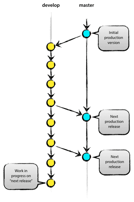 Image from: https://nvie.com/posts/a-successful-git-branching-model/
By always keeping the main branch clean, we can easily flag our CI/CD pipeline to be triggered as soon as we push to the main. We will be also free to commit as much as we need in the develop branch while we improve our models.
When we are ready for a new deploy we will only need to merge with the main branch (or better yet do a merge-request / pull-request and then merge).
This merge to main should trigger Gitlab to upload the new version of our model to the package registry.
Let's take a look at the simple way to automate publishing to the package registry using the .gitlab-ci.yml file.
CI/CD Pipeline
The .gitlab-ci.yml file is a special file in your repository used by Gitlab to define what the Gitlab server should do when you push to a repository.
To learn more about how CI/CD works in Gitlab, head over to this Gitlab CI/CD crash course.
In this tutorial our .gitlab-ci.yml file looks like this:
image: pytorch/pytorch

variables:
  VERSION: "0.0.4" # To Change if needs be

stages:
  - upload

upload:
  stage: upload
  only:
    - master
  script:
    - apt-get update
    - apt-get install -y curl wget
    - 'curl --header "JOB-TOKEN: $CI_JOB_TOKEN" --upload-file ./model.pth "${CI_API_V4_URL}/projects/${CI_PROJECT_ID}/packages/generic/example-ml-packaging-pipeline/${VERSION}/model.pth"'
    - 'curl --header "JOB-TOKEN: $CI_JOB_TOKEN" --upload-file ./run_mnist.py "${CI_API_V4_URL}/projects/${CI_PROJECT_ID}/packages/generic/example-ml-packaging-pipeline/${VERSION}/run_mnist.py"'
    - 'curl --header "JOB-TOKEN: $CI_JOB_TOKEN" --upload-file ./requirements.txt "${CI_API_V4_URL}/projects/${CI_PROJECT_ID}/packages/generic/example-ml-packaging-pipeline/${VERSION}/requirements.txt"'
    - 'curl --header "JOB-TOKEN: $CI_JOB_TOKEN" --upload-file ./INSTRUCTION.md "${CI_API_V4_URL}/projects/${CI_PROJECT_ID}/packages/generic/example-ml-packaging-pipeline/${VERSION}/INSTRUCTION.md"'
The anatomy of this .yml file is very bare bones. We have only one stage in our pipeline which is the upload stage.
In the upload stage, we will run the script section only when the master branch gets updated. The script that we ran is simply using curl to transfer the data from this repository (4 files) into the package registry.
Let's take a look at the anatomy of the curl command we are using:
- 'curl --header "JOB-TOKEN: $CI_JOB_TOKEN" --upload-file ./NAME_OF_FILE "${CI_API_V4_URL}/projects/${CI_PROJECT_ID}/packages/generic/example-ml-packaging-pipeline/${VERSION}/NAME_OF_FILE"'
--headeris used to tell curl that you will be including an extra header to the request.JOB-TOKENis our header and$CI_JOB_TOKENis its value. It's a variable that lives within Gitlab servers when a job is created--upload-fileis a flag to tell that we will transfer a local file to the remote URL../NAME_OF_FILEis the name of the local file we want to transfer.${CI_API_V4_URL}/projects/${CI_PROJECT_ID}/packages/generic/example-ml-packaging-pipeline/${VERSION}/NAME_OF_FILEis the location of the remote URL that we want to transfer a file.
Here $CI_API_V4_URL is the URL of the Gitlab API we are using, $CI_PROJECT_ID is defined within Gitlab CI as the id for our project, and finally VERSION is the version number we defined at the top of the .yml file.
That's it! When you update the main branch to the remote repository on Gitlab it will fire up a pipeline that will run your packaging job.
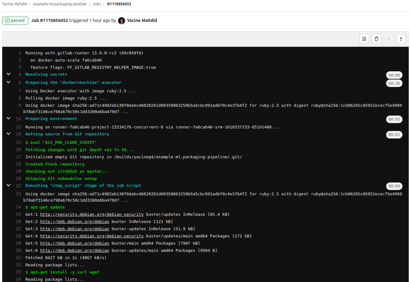 The job will then be available and you will be able to check the trace on Gitlab!
You and your teammates will be able to see the document in the package registry section and get the right versioned files in the package:
 This is our v.0.0.5 of the example package!
To get a more complete idea of what is possible with the Packages API, head over to the official documentation.
Conclusion
In this tutorial you've learn how to bundle, upload, and automatize a machine learning model packaging using Gitlab CI/CD.
Congratulation! 🎉🎉🎉
There is still a lot more you can do with Gitlab CI/CD, for instance:
- Add a testing stage before the bundling in order to make sure that there is no regression in the code.
- Add a testing stage after the bundling to make sure that the performance of your model is satisfactory in terms of inference latency.
- Use a more optimized version of the model with TorchScript.
- Add automatic social notification of new release after the upload step.
To learn more about Gitlab CI/CD the official docs is a great place to start out, and the get started section is very beginner friendly.
If you want to read more of this type of content, check out my mechanical/software engineering articles. If you want to discuss any of this feel free to send me a DM on LinkedIn or Twitter :)