
Recently, there's been a massive amount of effort put into developing novel image processing techniques. And many of them are derived from digital signal processing methods such as Fourier and Wavelet transforms.
These techniques have not only enabled a wide range of image processing techniques such as noise reduction, sharpening, and dynamic-range extension, but have also enabled many techniques used in compute vision such as edge detection, object detection, and so on.
Multi-scale analysis is one of the newer techniques (relatively speaking) that has been adopted in a wide range of applications, especially in the astronomical image and data processing applications. This technique, which is based on Wavelet transform, allows us to divide our data into multiple signals, that all add up to make the final signal.
We can then perform our processing or analysis work on this individual sub-signals, allowing us to do targeted operations that do not affect other sub-signals.
In this tutorial, we'll first be exploring what the technique is all about, through the lens of a particular algorithm for performing multi-scale analysis on images. We'll then move on to looking at how we can implement what we discussed in the first part in Rust programming language and recreate the examples you see in the first half of the article.
Before You Read:
Prerequisites for Part 1:
The technique described is derived from the concept of "Wavelet Transforms". You don't need to know everything about it, but a very basic understanding will help you grasp the material better.
Since the article focuses on image processing and analysis, a basic understanding of how pixels work in digital format is helpful, but not mandatory.
Prerequisites for Part 2:
Here, we focus on implementing the algorithm using the Rust programming language, without going much into the details of the language itself. So being comfortable writing Rust programs, and comfortable reading crate documentations is required.
If this is not you, you can still read Part 1 and learn the technique, and then maybe you'll want to then try it out in a language of your choice. If you're not familiar with Rust, I highly encourage you to learn the basics. Here's an interactive Rust course that can get you started.
Table Of Contents
- Part 1: Understanding Multi-Scale Processing Technique And Algorithm
- Part 2: How to Implement À Trous Tranform in Rust
- Wrapping Up
Part 1: Understanding the Multi-Scale Processing Technique and Algorithm
So what do we mean when we talk about multi-scale processing or analysis of some data? Well, we usually mean breaking down the input data into multiple signals, each representing a particular scale of information.
Scale, when talking about image analysis, simply refers to the size of structures that we are looking at at any given time. It ignores everything else that's either smaller or larger than the current scale.
What is multi-scale image processing?
For images, "scales" generally refer to the size in pixels of various structures or details in the image. You'll be able to get an intuitive understanding by looking at the following example:
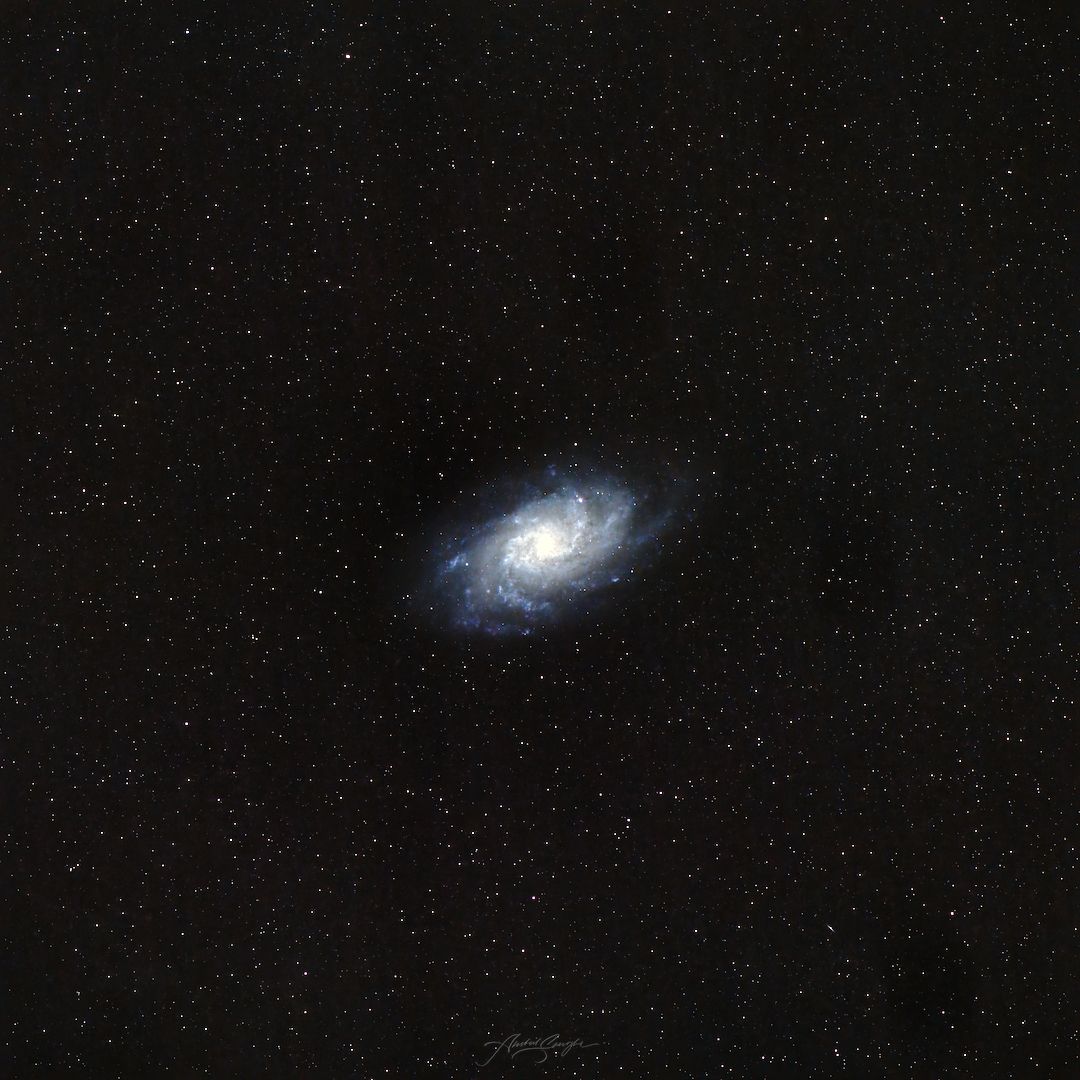 Messier 33, AKA Triangulum Galaxy
Assuming our naïve understanding is correct, we can derive images of at-least the following 3 scales:
- Very small structures, usually the size of a single pixel. This layer, when separated from the rest of the image, will only contain the noise and some sharp stars for the most part.
- Small structures, usually a few pixels in size. This layer, when separated, will contain all of the stars and the very fine details in the galaxy arms.
- Large and very large scale structures, usually 100s of pixels in size. This layer, when separated, will contain the general size and shape of the galaxy at the center.
Now the question becomes, why do we need to do all of this in the first place?
The answer is simple: it allows us to make targeted enhancements and changes to an image.
For example, noise reduction on the overall image will usually result in a loss of sharpness in the galaxy. But since we have broken our image down into multiple scales, we can easily apply noise reduction to only the first few layers, as most of the random noise that is easy to remove resides only in lower scale layers.
We then re-combine the noise-reduced low-scale layers with unmodified large-scale ones, and we have an output that gives us noise reduction without a loss in quality.
Another peculiar thing about noise is that it's almost always present in just one of these layers, making noise reduction process both easy and non-destructive.
If you're more of a visual learner, let's see this in practice using the image we used above. We're gonna be working with the following grayscale version of that image, where I've also added random gaussian noise:
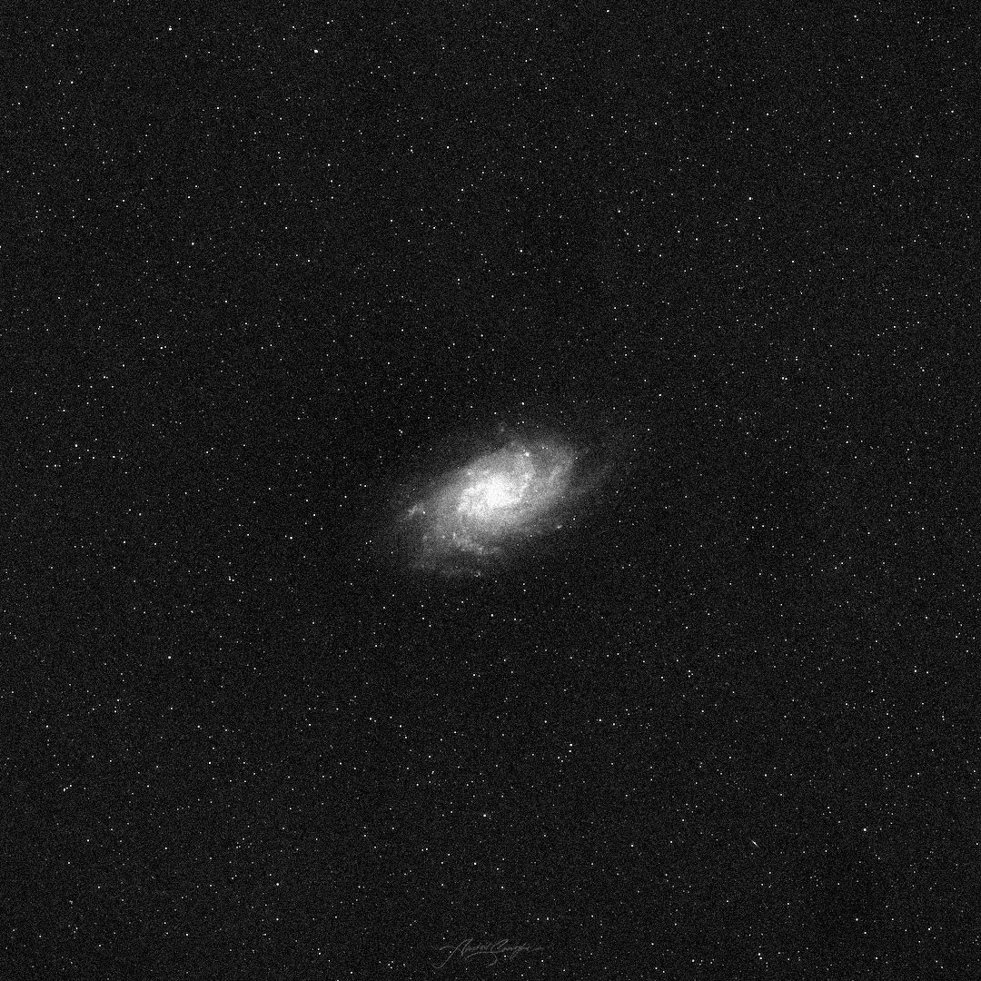 Messier 33 AKA Triangulum Galaxy, Converted to grayscale and with added Gaussian noise
Performing scale-based layer separation on this image, we get the following results. Note that the results are rescaled to a range where they can be viewed as an image for representational purpose. The actual transform produces pixel values that don't make sense when looked at independently, but all of the techniques and calculations described in this tutorial can still be safely applied without rescale. The recomposition process automatically gives us back the correct range:
 9-level À Trous Decomposition. From top-left to bottom-right, we have images at the following pixel scales: 1, 2 4, 8, 16, 32, 64, 128, 256 (powers of 2)
- The first and second layers contain the noise and stars. In this particular example, noise is mixed in with the stars. But using the first and second layers, we can easily target areas that are not present in the second layer, as we can be sure that those are where the noise is present in the first layer.
- With the third layer, we still see the residue luminance from stars. But if you look closely, we also see very faintly the arms of the galaxy starting to appear.
- From the fourth layer onwards, we see the galaxy at varying scales and detail levels, completely without the stars. We start with the finer details (relatively small scale details) and increasingly move on to larger and larger scale samples. By the end, we only see a vague shape where the galaxy used to be.
From here on, we can selectively apply noise reduction to the first two layers. Then we can recombine all of the layers to create the following image that has very little noise while preserving the same amount of details in the stars and the galaxy arms:
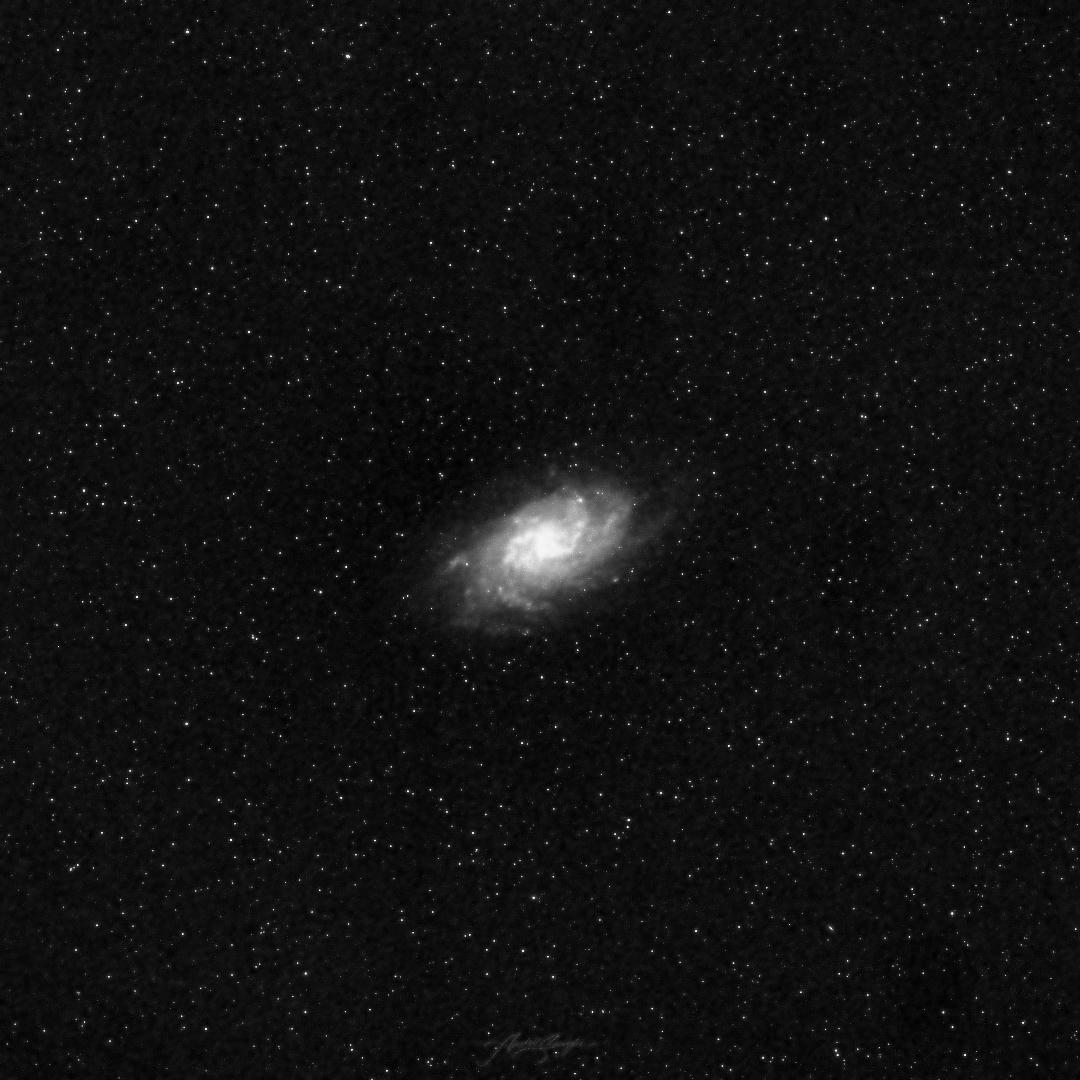 Messier 33 AKA Triangulum Galaxy, result of recombining all layers but with noise reduction applied to the pixel scale 1 & 2 layers
In its most basic form, multi-scale analysis involves breaking up your source image, commonly referred to as the "signal", into multiple "signals" – each containing the data for a particular scale in the source signal.
Scale, when talking about image signal here, refers to the distance between adjacent pixels that we take when creating the layer from the source image.
In practice, this technique is used as the one of the first steps in all kinds of astronomical data analysis and image processing.
As an example, you can use the technique to detect locations of stars while ignoring larger structures much more easily than would be possible otherwise.
The À Trous Wavelet Transform
All of what I've showed you previously, and all of what you're going to see in this tutorial, was achieved with wavelet decomposition and recomposition using the à trous algorithm for discreet wavelet transforms.
This algorithm has been used throughout the years for various applications. But it's become particularly important recently in astronomical image processing applications, where different objects and signals in an image can be completely separated based on structural scales.
Here's how the algorithm works:
- We start with the source image input and number of levels to decompose into n.
- For each level n:
- We convolve the image with our scaling function (we'll see what this is in a bit), where adjacent pixels are considered to be 2n units apart from each other, giving us the result resultn. This is where the "À Trous" name comes from, which literally translates to "with holes".
- The layer output outputn is then computed using input - resultn.
- We then update input to equal resultn. This is also known as residue data which serves as the source data for next layer.
- Repeat the above steps for all levels.
- In the end, we have 9 wavelet layers, and 1 residue layer. All 10 layers are required for the recomposition.
For a more mathematical approach to understanding this algorithm, I encourage you to read about the à trous algorithm here.
The recomposition process is very straightforward: we just need to add all 10 layers together. We can chose to apply positive or negative bias to any of the layers, which is a factor by which to multiply the layer pixel values during recomposition. You can use it either to enhance or diminish the characteristics of that particular layer.
Scaling Functions
Scaling functions are specific convolution kernels that help us better represent data at a particular scale based on our use case. There are 3 most commonly used scaling functions, which are shown below:


The images above show the 3 most commonly used scaling functions in the À Trous algorithm, visualised using 3rd level decomposition of the triangulum galaxy image used previously:
- B3 Spline is a very smooth kernel. It is mostly used in isolation of large scale structures. If we wanted to sharpen our galaxy, we would have used this kernel.
- Low-scale is a very sharply peaked kernel, and is best at working with small scale structures.
- Linear interpolation kernel gives us the best of both worlds, and hence is used when we need to work with both small scale and large scale structures. This is what we have used in all of our previous examples.
Convolution Pixels At Each Scale
I mentioned in the algorithm that at each scale, the pixels in the image are considered to be 2n units apart. Let's try to grasp a better understanding of this using the following visualisation:
Consider the following 8px by 8px image. Each pixel is labeled 1 through 64, which is their index.
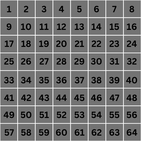 A representational pixel grid of a 8x8px image
We're going to focus on a convolution operation of one of the center pixels only for this example, let's say pixel number 28.
Scale 0: At scale 0, the value of 2n becomes 1. This means that for convolution, we'll consider pixels that are 1 unit apart from our target center pixel. These pixels are highlighted below:
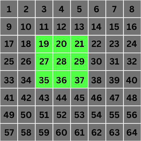 8x8px grid with pixels that are involved in convolution for pixel number 28 highlighted at scale 0
Scale 1: This is where things get interesting. At scale 1, the value of 2n becomes 2. This means that for convolution, we'll jump directly to pixels that are 2 locations apart from the target pixel:
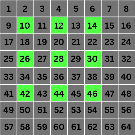 8x8px grid with pixels that are involved in convolution for pixel number 28 highlighted at scale 1
As you can see, we've created "holes" in our computation of the value of the target pixel by skipping 2n - 1 adjacent pixels and selecting the 2nth pixel. This is the basis of the algorithm.
This process is repeated for every pixel in the image, just like a regular convolution process. And each time, we consider increasing distances between pixels for computation of final values at increasing scales.
Let's look at just one more scale.
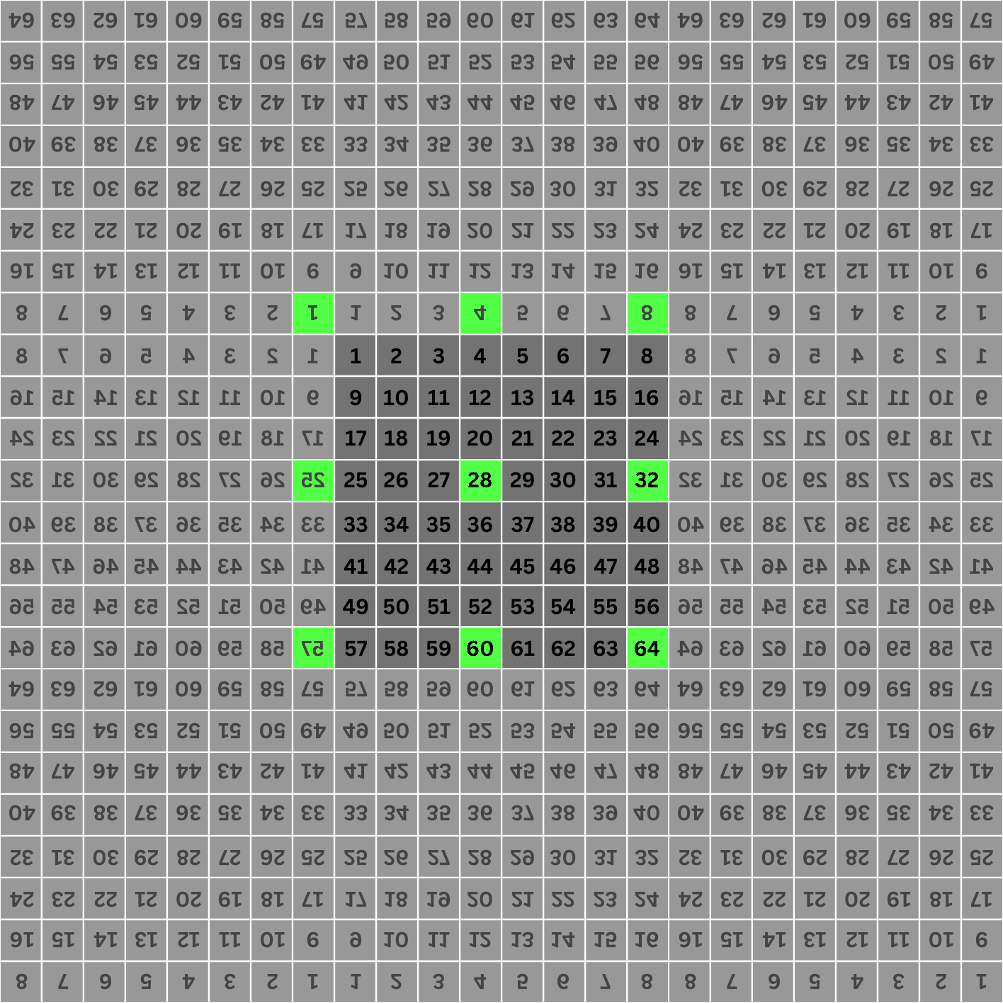
Scale 2: This is where things get even more interesting. At scale 2 the value of 2n becomes 4. This means that for convolution, we'll jump directly to pixels that are 4 locations apart from the target pixel:
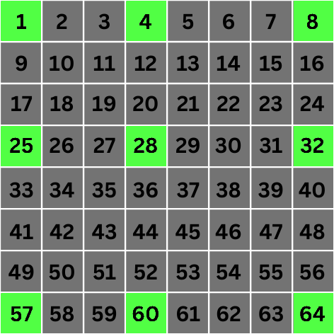 8x8px grid with pixels that are involved in convolution for pixel number 28 highlighted at scale 2
Wait what? Why are we choosing pixels 1, 4, 8, 25, & 57? 1 & 4 are only 3 locations apart, 25 is only 2 locations apart, and 8 & 57 are not even diagonally aligned with the target pixel. What's going on?
Handling Boundary Conditions
As we've mentioned that this process is executed for all of the pixels in an image, we also need to consider cases where the pixel locations for convolution lie outside of the image.
This is not a concept unique to this algorithm. During convolution, this is referred to as a boundary condition or handling boundary pixels. There are various techniques for dealing with this, and all of them involve virtually extending the image in order to make it seem like we're not encountering the boundary at all.
Some of the techniques are:
- Extending as much as needed by copying the value of the last row/column
- Mirroring the image on all edges and corners
- Wrapping the image around the edges.
In our example, we're employing the "mirroring" technique. When implementing such an algorithm, we don't need to actually create an extended image. Any boundary handling is implementable using just basic mathematical formulae.
Our extended image, with the correct pixels selected for scale 2, is as follows:
 Source image extended on all edges and corners using the mirroring technique. All of the faded regions represent extended areas.
Again, the extension is only logical and is completely computed using formulae, as opposed to actually extending the source image and then checking. We can easily see that with the mirrored images in place, our basic rule of picking pixels that are 2n locations apart is still followed.
Computing Maximum Possible Scales for Any Given Image
If you think about it carefully, you'll see that the maximum layers an image can be decomposed into can be calculated by computing the log2 of the image width or height (whichever is lower) and throwing away the fractional part.
In our 5x5 image, log2(5) ~= 2.32. If we throw away the fractional part, that leaves us with 2 layers. Similarly, for a 1000x1000px image, log21000 ~= 9.96, which means we can decompose a 1000x1000 px image into a maximum of 9 layers. It simply implies that our "holes" cannot be larger than the width or height.
Even with the mirroring extension we used above, if the holes are larger than the width of the image, they'll still end up outside of the extended regions, specially for corner or boundary pixels, making it impossible to perform convolution at that scale.
Closing Notes
Thinking about the examples and visualisations a bit more, you can clearly see how and why this algorithm works, and how it's able to separate out structures in an image based on their sizes. The increasing hole sizes make it so that only structures larger than the hole itself are retained for any given layer.
A big advantage of using this algorithm is the computational cost. Since this doesn't involve Fourier or Wavelet transforms, the computational cost is quite low, relatively speaking. The memory cost, however, is indeed higher. But more often than not that is a good tradeoff.
Another advantage of this algorithm when comparing it to other discreet wavelet transform algorithms is that the size of source image is preserved throughout the entire process. There's no decimation or upscaling happening here, making this algorithm one of the easiest ones to understand and implement.
The algorithm is used in almost all of the astronomical image processing softwares such as PixInsight, Siril, and many others.
This algorithm is also known by other names such as Stationary Wavelet Transform and Starlet Transform.
Part 2: How to Implement À Trous Tranform in Rust
Now I'm going to show you how you can implement this algorithm in Rust.
For the purposes of this tutorial, I'm going to assume that you're pretty familiar with Rust and its basic concepts, such as data-types, iterators, and traits and are comfortable writing programs that use these concepts.
I'm also going to assume that you have an understanding of what convolution and convolution kernels mean in this context.
Prerequisites
We're going to need a couple of dependencies. Before we get to that, let's quickly create a new project:
cargo new --lib atrous-rs
cd atrous-rs
Now let's all of the dependencies we need. We actually only need 2:
cargo add image ndarray
image is a Rust library we'll use to work with images of all of the standard formats and encodings. It also helps us convert between various formats, and provides easy access to pixel data as buffers.
ndarray is a Rust library that helps you you create, manipulate, and work with 2D, 3D, or N-Dimensional arrays. We can use nested Vectors, but using a project like ndarray is better in this case because we need to perform a lot of operations on both individual values as well as their neighbours. Not only is it much easier to do with ndarray, but they also have performance optimisations built in for many operations and CPU types.
Although I'll be covering the basic functions/traits/methods/data-types we use from these crates, I'm not going to go into too much detail for them. I encourage you to read the docs instead.
We're actually going to jump straight to algorithm implementation, and come back later to see how we can use it.
The À Trous Transform
Create a new file that will hold our implementation. Let's name it transform.rs.
Start with adding the following struct, that will hold the information we need to perform the transform:
// transform.rs

use ndarray::Array2;

pub struct ATrousTransform {
    input: Array2<f32>, // `Array2<f32>` is a 2D array where each value is of type `f32`. This will hold our pixel data for input image.
    levels: usize, // The number of levels or scales to decompose the image into
    current_level: usize, // Current level that we need to generate. This holds the state of our iterator.
    width: usize, // Width of input image
    height: usize, // Height of input image
}
We also need a way to create this struct easily. In our case, we want to be able to create it from the input image directly. Also, input image can be of any of the supported format and encoding, but we want a consistent color-type to implement the calculations, so we'll also need to convert the image to our expected format.
It's helpful to extract all of this logic away using the "constructor" pattern in Rust. Let's implement that:
// transform.rs

use image::GenericImageView;

impl ATrousTransform {
    pub fn new(input: &image::DynamicImage, levels: usize) -> Self {
        let (width, height) = input.dimensions();
        let (width, height) = (width as usize, height as usize);

        // Create a new 2D array with proper size for each dimension to hold all of our input's pixel data. Method `zeros` takes a "shape" parameter, which is a tuple of (rows_count, columns_count).
        let mut data = Array2::<f32>::zeros((height, width));

        // Convert the image to be a grayscale image where each pixel value is of type `f32`. Loop over all pixels in the input image along with its 2D location.
        for (x, y, pixel) in input.to_luma32f().enumerate_pixels() {
            // Put the pixel value at appropriate location in our data array. The `[[]]` syntax is used to provide a 2-dimensional index such as `[[row_index, col_index]]`
            data[[y as usize, x as usize]] = pixel.0[0];
        }

        Self {
            input: data,
            levels,
            current_level: 0,
            width,
            height
        }
    }
}
This takes care of converting the image to grayscale and converting the pixel values to f32. If you're not already aware, for images with floating-point pixel values, the values are always normalized. This means that they are always between 0 and 1 – 0 representing black and 1 representing white.
Iterators and the À Trous Transform
Before we continue, let's think about the algorithm for a second. We need to be able to generate images at increasing scales, until we hit the maximum number of levels we need.
We want the consumer of our library to have access to all of these scales, and be able to manipulate them and also easily recombine once they're done. They need to be able to filter layers to ignore structures at certain scales, manipulate or "map" them to change their characteristics, perform operations on them, or even store each image if they so need.
This sounds an awful lot like Iterators! Iterators give us methods like filter, skip, take, map, for_each, and so on, all of which are exactly all we need to work with our layers before recomposition.
One added advantage of Iterators is that it allows you to finish processing each layer all the way through before you move on to the next one. If you're unsure why this is, I suggest reading more about processing a series of items with Iterators in Rust.
We're going implement the Iterator trait for our ATrousTransform type which should produce a wavelet layer as output for each iteration.
We're going to be implementing the inner-most parts of the algorithm first, and build out from there. So we first need a way to convolve an input data buffer with the scaling function while making sure that adjacent pixels are 2n locations apart, which is the first step in our loop.
Convolution
We need to define our convolution kernel before we can do anything else. Create a new file kernel.rs and add it to lib.rs with the following contents:
// kernel.rs

#[derive(Copy, Clone)]
pub struct LinearInterpolationKernel {
    values: [[f32; 3]; 3]
}

impl Default for LinearInterpolationKernel {
    fn default() -> Self {
        Self {
            values: [
                [1. / 16., 1. / 8., 1. / 16.],
                [1. / 8., 1. / 4., 1. / 8.],
                [1. / 16., 1. / 8., 1. / 16.],
            ]
        }
    }
}
We define it using a struct instead of a constant array of arrays because we need to define some tiny helpful methods on it related to index handling. We'll come back to that later.
Create another file convolve.rs. This is where all of the code for handling convolution for individual pixels will go. We'll define a Convolution trait that will define methods needed to perform the convolution on every pixel in current layer.
// convolve.rs

pub trait Convolution {
    fn compute_pixel_index(
        &self,
        distance: usize,
        kernel_index: [isize; 2],
        target_pixel_index: [usize; 2]
    ) -> [usize; 2];

    fn compute_convoluted_pixel(
        &self,
        distance: usize,
        index: [usize; 2]
    ) -> f32;
}
You may ask why we need a trait here instead of a simple impl block. We are only working with Grayscale images in this article, but you may want to extend it to implement it for RGB or other color modes as well.
Now, you need to implement this trait for your ATrousTransform struct:
// convolve.rs

impl Convolution for ATrousTransform {
    fn compute_pixel_index(
        &self,
        distance: usize,
        kernel_index: [isize; 2],
        target_pixel_index: [usize; 2]
    ) -> [usize; 2] {
        let [kernel_index_x, kernel_index_y] = kernel_index;

        // Compute the actual distance of adjacent pixel
        // by multiplying their relative position with the
        // size of the hole.
        let x_distance = kernel_index_x * distance as isize;
        let y_distance = kernel_index_y * distance as isize;

        let [x, y] = target_pixel_index;

        // Compute the index of adjacent pixel in the 2D
        // image based on the index of current pixel.
        let mut x = x as isize + x_distance;
        let mut y = y as isize + y_distance;

        // If x index is out of bounds, consider x to be
        // the nearest boundary location
        if x < 0 {
            x = 0;
        } else if x > self.width as isize - 1 {
            x = self.width as isize - 1;
        }

        // If y index is out of bounds, consider y to be
        // the nearest boundary location
        if y < 0 {
            y = 0;
        } else if y > self.height as isize - 1 {
            y = self.height as isize - 1;
        }

        // The final 2D index of pixel.
        [y as usize, x as usize]
    }

    fn compute_convoluted_pixel(
        &self,
        distance: usize,
        [x, y]: [usize; 2]
    ) -> f32 {
        // Create new variable to hold the result of convolution
        // for current pixel.
        let mut pixels_sum = 0.0;

        let kernel = LinearInterpolationKernel::default();

        // Iterate over relative position of pixels from the center
        // pixel to perform convolution with. In other words,
        // these are the indexes of neighbouring pixels from the
        // center pixel.
        for kernel_index_x in -1..=1 {
            for kernel_index_y in -1..=1 {
                // Get the computed pixel location that maps to
                // the current position in kernel
                let pixel_index = self.compute_pixel_index(
                    distance,
                    [kernel_index_x, kernel_index_y],
                    [x, y]
                );

                // Get the multiplicative factor (kernel value) for
                // this relative location from the kernel.
                let kernel_value = kernel.value_from_relative_index(
                    kernel_index_x,
                    kernel_index_y
                );

                // Multiply the pixel value with kernel scaling
                // factor and add it to the pixel sum.
                pixels_sum += kernel_value * self.input[pixel_index];
            }
        }

        // Return the value of computed pixel from convolution process.
        pixels_sum
    }
}
We need to do computations to figure out each pixel's location based on the relative position in the kernel from the center pixel as well as ensure that the "hole size" is also being taken into consideration for the final pixel index. As you might notice, you also want to handle the boundary conditions when computing indexes.
I encourage to take your time here and go through the code and the comments.
Implementing the Iterator
It's finally time to implement the Iterator trait for your ATrousTransform:
// transform.rs
impl Iterator for ATrousTransform {
// Our output is an image as well as the current level for each
// iteration. The current level is an `Option` to represent the
// final residue layer after the intermediary layers have been
// generated.
type Item = (Array2::<f32>, Option<usize>);
fn next(&mut self) -> Option<Self::Item> {
let pixel_scale = self.current_level;
self.current_level += 1;
// We've already generated all the layers. Return None to
// exit the iterator.
if pixel_scale > self.levels {
return None;
}
// We've generated all intermediary layers, return the
// residue layer.
if pixel_scale == self.levels {
return Some((self.input.clone(), None))
}
let (width, height) = (self.width, self.height);
// Distance between adjacent pixels for convolution (also
// referred to as size of "hole").
let distance = 2_usize.pow(pixel_scale as u32);
// Create new buffer to hold the computed data for this layer.
let mut current_data = Array2::<f32>::zeros((height, width));
// Iterate over each pixel location in the 2D image
for x in 0..width {
for y in 0..height {
// Set the current pixel in current layer to
// the result of convolution on the current
// pixel in input data.
current_data[[y, x]] = self.compute_convoluted_pixel(
distance,
[x, y]
);
}
}
// Create current layer by subtracting currently computed pixels
// from previous layer
let final_data = self.input.clone() - ¤t_data;
// Set the input layer to equal the current computed layer so
// that it can be used as the "previous layer" in next iteration.
// This is also our residue data for each layer.
self.input = current_data;
// Return the current layer data as well as current level information.
Some((final_data, Some(self.current_level)))
}
}
I'm going to point out that there's a lot of potential for optimizing for performance here, but that's out of the scope of this article.
We'll finally look at how we can take all of these layers and reconstruct our input image.
Recomposition
As I've said previously, reconstructing an image that was decomposed with the A Trous transform is as simple as summing all of the layers together.
We're going to define a trait for this. Why we need a trait here should be clear once you look at the implementation.
Create a new file recompose.rs with the following contents:
// recompose.rs

use image::{DynamicImage, ImageBuffer, Luma};
use ndarray::Array2;

pub trait RecomposableLayers: Iterator<Item = (Array2<f32>, Option<usize>)> {
    fn recompose_into_image(
        self,
        width: usize,
        height: usize,
    ) -> DynamicImage
        where
            Self: Sized,
    {
        // Create a result buffer to hold the pixel data for our output image.
        let mut result = Array2::<f32>::zeros((height, width));

        // For each layer, add the layer data to current value of result buffer.
        for layer in self {
            result += &layer.0;
        }

        // Compute min and max pixel intensity values in the final data so that
        // we can perform a "rescale", which normalizes all pixel values to be
        // between the range of 0 & 1, as is expected by float 32 images.
        let min_pixel = result.iter().copied().reduce(f32::min).unwrap();
        let max_pixel = result.iter().copied().reduce(f32::max).unwrap();

        // Create a new `ImageBuffer`, which is a type provided by `image` crate to
        // serve as buffer for pixel data of an image. Here, we're creating a new
        // `Luma` ImageBuffer with pixel value of type `u16`. Luma just refers to
        // grayscale.
        let mut result_img: ImageBuffer<Luma<u16>, Vec<u16>> =
            ImageBuffer::new(width as u32, height as u32);

        // Pre-compute the denominator for scaling computation so that we don't
        // repeat this unnecessarily for every iteration.
        let rescale_ratio = max_pixel - min_pixel;

        // Iterate over all pixels in the `ImageBuffer` and fill it based on data
        // from the `result` buffer after rescaling the value.
        for (x, y, pixel) in result_img.enumerate_pixels_mut() {
            let intensity = result[(y as usize, x as usize)];

            *pixel =
                Luma([((intensity - min_pixel) / rescale_ratio * u16::MAX as f32) as u16]);
        }

        // Convert the `ImageBuffer` into `DynamicImage` and return it
        DynamicImage::ImageLuma16(result_img)
    }
}

// Implement this trait for anything that implements the Iterator trait
// with the given item type
impl<T> RecomposableLayers for T where T: Iterator<Item = (Array2<f32>, Option<usize>)> {}
If you haven't noticed, since we implement this trait for a generic, this will work with any iterator, such as Filter, Map, and so on. If you didn't use a trait here, you'll have had to implement the same thing again and again for every built-in iterator type, and your code wouldn't have worked with 3rd party types.
Using the À Trous Transform
After all of that, it's finally time to reproduce the processing that I showed you for the galaxy image with lots of noise. Create a new file main.rs with the following contents:
use image::{DynamicImage, ImageBuffer, Luma};
use atrous::recompose::RecomposableLayers;
use atrous::transform::ATrousTransform;

fn main() {
    // Open our noisy image
    let image = image::open("m33-noise-lum.jpg").unwrap();

    // Create a new instance of the transform with 9 layers
    let transform = ATrousTransform::new(&image, 9);

    // Map over each layer
    transform.map(|(mut buffer, pixel_scale)| {
        // Create a new image buffer to hold the pixel data. This
        // will be populated from the raw buffer for this layer.
        let mut new_buffer =
            ImageBuffer::<Luma<u16>, Vec<u16>>::new(buffer.ncols() as u32, buffer.nrows() as u32);

        // Iterate over all pixels of the `ImageBuffer` to populate it. We also
        // convert from `f32` pixels to `u16` pixels.
        for (x, y, pixel) in new_buffer.enumerate_pixels_mut() {
            *pixel = Luma([(buffer[[y as usize, x as usize]] * u16::MAX as f32) as u16])
        }

        // If the present layer is a small scale layer (< 3),
        // perform noise reduction
        if pixel_scale.is_some_and(|scale| scale < 3) {
            let mut image = DynamicImage::ImageLuma16(new_buffer).to_luma8();

            // Bilateral filter is a de-noising filter. Apply it to the image.
            image = imageproc::filter::bilateral_filter(&image, 10, 10., 3.);

            // Modify the raw buffer to contain the updated pixel values after
            // filtering.
            for (x, y, pixel) in image.enumerate_pixels() {
                buffer[[y as usize, x as usize]] = pixel.0[0] as f32 / u8::MAX as f32;
            }

            // Return the updated buffer.
            (buffer, pixel_scale)
        } else {
            // Return the unmodified buffer for larger scale layers.
            (buffer, pixel_scale)
        }
    })
        // Call the recomposition method on iterator
        .recompose_into_image(image.width() as usize, image.height() as usize)
        // Convert output to 8-bit grayscale image
        .to_luma8()
        // Save it to jpg file
        .save("noise-reduced.jpg")
        .unwrap()
}
You also need to add a new dependency, imageproc, which provides useful image processing implementations on top of the image crate.
cargo add imageproc
To make this work, we also need to modify our Cargo.toml to explicitly define both binary and library targets:
// Cargo.toml

[package]
name = "atrous-rs"
version = "0.1.0"
edition = "2021"

[[bin]]
name = "atrous"
path = "src/main.rs"

[lib]
name = "atrous"
path = "src/lib.rs"

# See more keys and their definitions at https://doc.rust-lang.org/cargo/reference/manifest.html

[dependencies]
image = "0.25.1"
imageproc = "0.24.0"
ndarray = "0.15.6"
You may download the test image from here. Move it to the root directory of your project, and run cargo run --release. Once it finishes, you should have a new file noise-reduced.jpg as the output of our process.
And there we have it.
Further Reading
These are some of the resources that were very helpful to me when I was learning about this algorithm and how to use it. I highly encourage anyone who wants a more technical understanding of the algorithm to check these out.
- The à trous algorithm
- The À Trous Discrete Wavelet Transform In PixInsight
- Astronomical Image and Data Analysis by Jean-Luc Starck and Fionn Murtagh
- Sparse Image and Signal Processing: Wavelets and Related Geometric Multiscale Analysis by J.L. Starck, F. Murtagh, and J. Fadili
In addition, I've created a Rust library for working with À Trous transform. It closely matches with what I've showed you here, but has some additional features already, and will have even more.
Things such as handling RGB images and working with all the 3 different kernels is already implemented. It also has better logic for handling boundary conditions, where it uses the image folding technique.
I'm also soon going to be working on performance improvements for the same.
If you want to learn more, or contribute to the library, feel free to do so. The repository can be found here: https://github.com/anshap1719/image-dwt
Wrapping Up
I hope you enjoyed the journey so far. If image processing techniques or their implementation in Rust is something that interests you, then stay tuned for more as these are the topics I love writing about.
Also, feel free to contact me if you have any questions or opinions on this topic.
Enjoying my work?
Consider buying me a coffee to support my work!
Till next time, happy coding and wishing you clear skies!