

Data analysis is an extremely valuable skill to have. But to make the most of your analysis, it's invaluable to get your data neat and orderly.
In this article, I'll show you how to combine several functions together to better organize your data.
 gif of toys talking to each other saying, data, data everywhere
Google Sheets and Microsoft Excel are fantastic training grounds for computer programming. They allow quick access to writing functions that help you creatively solve problems just like in "real" programming. And, they also offer immediate results with the ability to troubleshoot bugs.
Today we'll grab a sample dataset from Kaggle and use it to illustrate:
- Shortcomings of simple, built-in functions
- How to nest functions
- How to extract and count unique values from our dataset
The Data and the Problem
We're going to look at a dataset from Kaggle that was scrapped from IMDB. It's a list of 1000 movies. The piece we'll concern ourselves with is the genre column.
If you'd like to follow along, the dataset is here, I've built a spreadsheet here that you can follow along with and even make a copy of, and I've recorded a walkthrough video here:
The issue that we'll solve is this: in the genre column, we want to extract all the unique values and count the number of times the appear. So, how many movies have Drama as a genre, Action as a genre...and so on.
If each cell had only one genre in it, this would be a quick fix. The built-in functions =UNIQUE() and =COUNTIF would solve this for us quickly.
However, most of the movies have more than one genre associated with them:
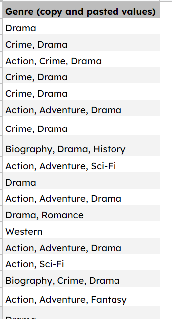 List of movie genres in a spreadsheet
If we try and use =UNIQUE(), we are going to be stuck because =UNIQUE() looks at each cell. So, it will think that the cell containing the value Crime, Drama is one unique value itself instead of knowing that it's a list of two genres.
Below is an example of what happens when using =UNIQUE() on a small portion of our dataset:
 using Unique function in spreadsheet
Luckily, spreadsheets are as smart as we're willing to make them. And we are able to use a combination of functions to extract the data we need.
Below, we'll walk through the steps and functions necessary to clean up and analyze our data properly.
The Functions We'll Use
First, let's take our dataset and get it into one big uniform list where every value is separated by commas since that's the issue above.
To do this, we'll use the =JOIN() function.
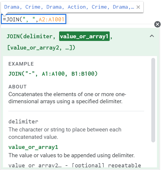 The join function in Google Sheets
=JOIN() lets us concatenate elements in our dataset with a delimiter – in our case, a comma and a space: =JOIN(", ",A2:A1001).
Next, we need to split that huge list so that we get all our values in their own cell. Recall, that this was the shortcoming initially because the =UNIQUE() function returns unique cells.
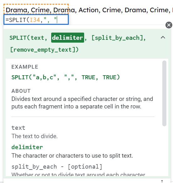 Split function in Google Sheets
The =SPLIT() function takes that huge list of comma-separated values and splits it into separate cells by whatever delimiter we specify. In this case, again, it'll be a comma and a space.
This would split everything across an incredibly long row, though.
So, we'll use the =TRANSPOSE() function to have it displayed down a column instead.
 Split and Transposed functions in Google Sheets
And we're in business. We can now use our original =UNIQUE() function to grab those unique values...and as an added bonus, the =SORT() function to get them alphabetically sorted.
 gif of man rejoicing quietly
How to Nest the Functions
Now that we know what all these do, let's nest them together in one cell to extract those unique values and sort them in a list in one fell swoop:
=UNIQUE(SORT(TRANSPOSE(SPLIT(JOIN(", ",A2:A),", ",FALSE))))
 gif of girl saying boom
Just like in algebra, we nest the functions that we need evaluated first deeper in the statement. So we have the =JOIN() function wrapped in the =SPLIT() function which is itself wrapped in the =TRANSPOSE() function, the =SORT() function and then finally at the very end, our =UNIQUE() function. The result is below:
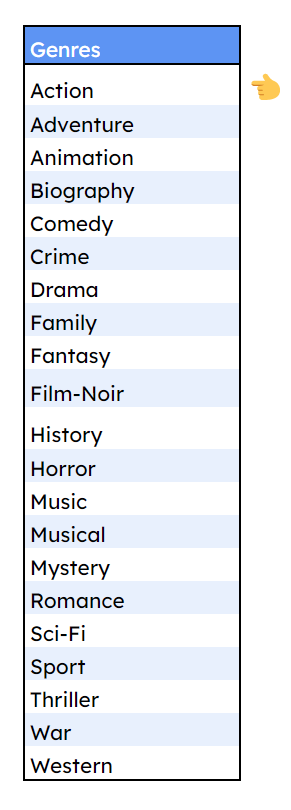 Complete sorted movie genre list
A Shorter Nested Function
From here, we can now count the occurrences of each genre in our main list using the =COUNTIF() function in a similar, though smaller nest.
We need to split and join our list first just like we did in the above example: =SPLIT(JOIN(", ",$A$2:$A),", ").
This becomes our range for the =COUNTIF() function. Then we count the values in that range if they're equal to the cells that hold our unique genre values.
For the Action genre in cell E19, here's the =COUNTIF() function:
=COUNTIF(SPLIT(JOIN(", ",$A$2:$A),", "),E19)
This returns 189 as the number of times Action is in our dataset. And by copying the formula down for each of our genres, we now have the number of occurrences of each of the genres.
Note: make sure to lock the dataset reference in place when you copy the formula down by enclosing the cell references in dollar signs: $A$2:$A. If you don't, then when you copy the formula down, that reference will shift down too.
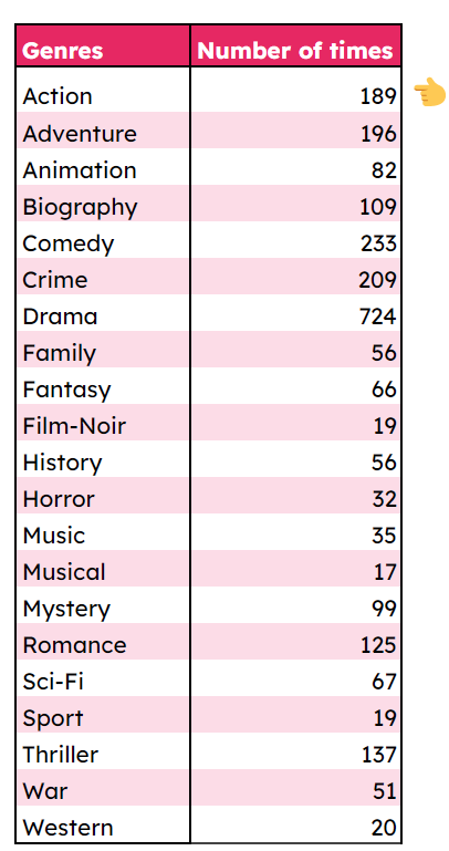 Number of times each genre appears in dataset
Conclusion
I hope this has been helpful for you! Spreadsheet functions are truly a great way to get into programming as well as expand your problem solving skills. I continue to enjoy optimizing my business by automating through spreadsheets.
📽️I'd love if you checked out my YouTube channel over here: https://www.youtube.com/@eamonncottrell
I'm making content like this all year and would appreciate a like/subscribe. Let me know what other videos/tutorials you'd benefit from!
💥You can also find me on Linkedin here: https://www.linkedin.com/in/eamonncottrell/
Have a great one! 👋