

Numerical analysis is the bridge between math and computer science.
Essentially, it is the development of algorithms that approximate solutions that pure math would also solve, but using less computational resources and faster.
This field is very important. Because for most solutions in the real world, we only need good approximations and not the exact solutions.
In this article, we will explore:
- Analogy Illustrating the Importance of Numerical Analysis
- Fundamentals of Numerical Analysis
- Application of Numerical Analysis in Real-World Problems
- Introduction to Partial Differential Equations (PDEs)
- Introduction to Optimization in Numerical Analysis
An Analogy that Illustrates the Importance of Numerical Analysis
How can we measure the coastline of an island?
If we try to measure every centimeter of every small segment, it would be impossible and probably time-consuming.
Because of the sea, the coastline is always changing at that level of detail.
However, by approximating and measuring in larger segments, we can get a practical measurement of the coastline.
This situation mirrors numerical analysis.
Approximation gives insights in situations where precise measurement is impossible or impractical.
Just as we accept a good estimation of the coastline length, numerical analysis uses approximation to solve hard problems.
Fundamentals of Numerical Analysis
Numerical analysis is all about approximation. It is like using binoculars to see a landscape that is very far away. We can't see every leaf. But we get a good enough picture to understand the terrain.
This is crucial in numerical analysis.
In this, we solve hard math problems where exact solutions are either impossible or extremely resource-intensive.
By approximating, we get sufficient good results with less computational effort.
Application of Numerical Analysis in Real-World Problems
There are many applications of numerical analysis
- In engineering, it enables simulation of structures and fluids.
- In finance, for risk assessment and portfolio optimization.
- In environmental science, it predicts climate patterns.
In each field, numerical analysis is a toolkit to solve problems where pure math just takes too much time, or it is impossible to give good results.
An Introduction to Partial Differential Equations (PDEs)
Partial Differential Equations (PDEs) are equations that describe how quantities like heat, sound, or electricity change in different places and as time goes on.
Solving PDEs is very important. Because it allows us to control these changes.
By allowing us to control them, we can:
- Predict weather patterns.
- Understand sound propagation in different environments.
- Design efficient transportation systems.
- Optimize energy distribution.
However, most PDE can only be approximated with numerical methods.
It is either too hard or impossible to find through normal calculations.
This way, with numerical methods, we are able to solve PDEs which in turn allows us to solve many real life problems.
Numerical Solutions of PDEs with SciPy
Solving PDEs with numerical methods often involves dividing the PDEs in small, manageable parts. Solve each one and then add them up.
SciPy, a Python library for scientific and technical computing, gives many tools for this purpose.
Now, let's solve a heat transfer problem in a rod.
In the below code, we will see line by line how it allows us to know how heat spreads in a rod:
import numpy as np
from scipy.integrate import solve_bvp

def heat_equation(x, y):
    return np.vstack((y[1], -y[0]))

def boundary_conditions(ya, yb):
    return np.array([ya[0], yb[0] - 1])

x = np.linspace(0, 1, 5)
y = np.zeros((2, x.size))

sol = solve_bvp(heat_equation, boundary_conditions, x, y)
Lets see how thhe code works block by block in the following sections.
How to importing libraries
import numpy as np
from scipy.integrate import solve_bvp
 Importing libraries
Here we import 2 python libraries:
These two python libraries are some of the most used in data science.
How to define the head equation and boundary conditions
def heat_equation(x, y):
    return np.vstack((y[1], -y[0]))

def boundary_conditions(ya, yb):
    return np.array([ya[0], yb[0] - 1])
 Defining heat equation and boundary conditions
We create heat_equation(x, y) and boundary_conditions(ya, yb).
In heat_equation(x, y) we are defining the differential equation we want to solve.
The boundary_conditions(ya, yb) function defines constrains at the start and end of a solution. The condition is that the end of the solution needs to be one unit less than the start.
How to solve the equation
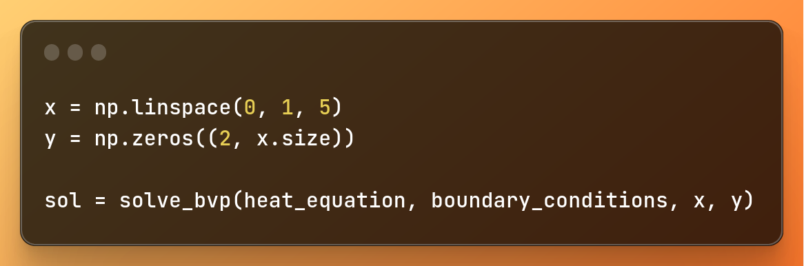
x = np.linspace(0, 1, 5)
y = np.zeros((2, x.size))

sol = solve_bvp(heat_equation, boundary_conditions, x, y)
 Solving equation
The line sol = solve_bvp(heat_equation, boundary_conditions, x, y) is the solution.
The code solve_bvp stands for solve boundary value problem.
It takes four arguments:
heat_equation: This is the main problem we are trying to solve.boundary_conditions: These are the mathematical constrains at the start and end of a solution.x: Are the spots we choose to explore our answers.y: Are initial attempts to solve the problem, based on your chosenxvalues.
An Introduction to Optimization in Numerical Analysis
Optimization is finding the best solution from all solutions. It is like finding the most efficient route in a complex network of roads.
Numerical optimization methods find the most efficient or cost-effective solution to a problem, whether that is:
- Minimizing waste in production.
- Maximizing efficiency in a logistic network.
- Finding best fit for a certain data model.
An Overview of Numerical Optimization Techniques with SciPy
The goal in this example is to minimize transportation cost across a network.
For instance, let's consider an optimization problem in logistics, where the goal is to minimize transportation cost across a network.
SciPy's minimize function can be used to find the best strategy to minimizes cost while meeting all constraints:
from scipy.optimize import minimize

def objective_function(x):
    return x[0]**2 + x[1]**2

def constraint_eq(x):
    return x[0] + x[1] - 10

con_eq = {'type': 'eq', 'fun': constraint_eq}

bounds = [(0, 10), (0, 10)]

x0 = [5, 5]

result = minimize(objective_function, x0, method='SLSQP', bounds=bounds, constraints=[con_eq])
Lets explain how the code works block by block.
How to importing the library
from scipy.optimize import minimize
 Importing scipy
Once again we import the necessary library:
How to defining objective and constraint equation
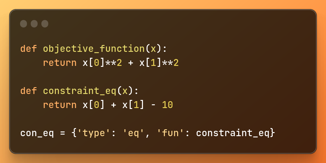
def objective_function(x):
    return x[0]**2 + x[1]**2

def constraint_eq(x):
    return x[0] + x[1] - 10

con_eq = {'type': 'eq', 'fun': constraint_eq}
 Define objective and constrain equations
- The objective function is the function we want to minimize to find the best answer.
- The constraint equation is the equation that limits the search space to those
xvalues that fulfill this equation.
con_eq is defined by the following:
'type': 'eq'indicates the type of constraint.'eq'means equality, in other words, the function must equal zero at the solution.'fun': constraint_eqassigns the constraint function.
We will see in the next block of code, it is where we constrain the possible solutions of the problem.
How to define an initial condition and result
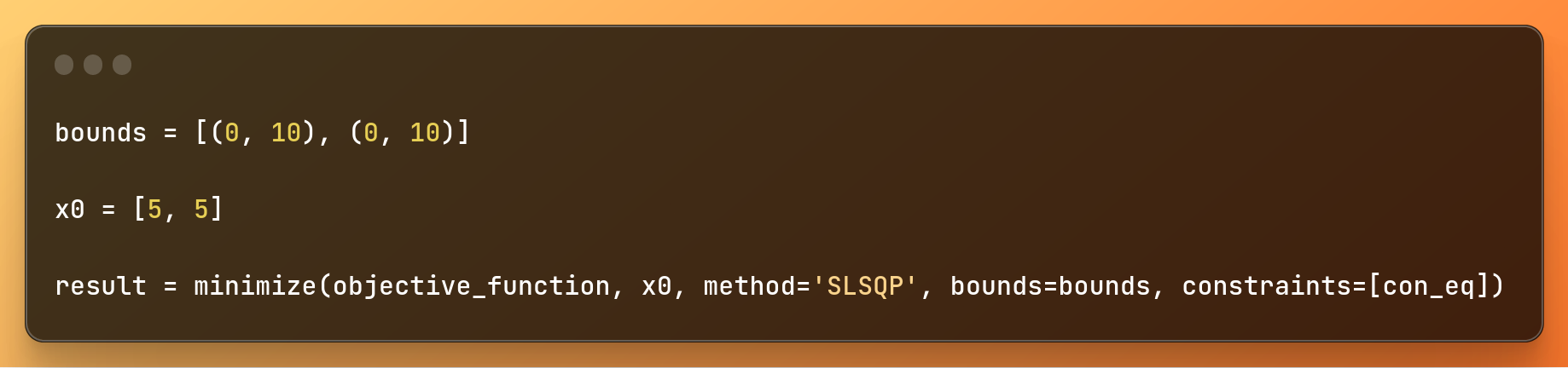
bounds = [(0, 10), (0, 10)]

x0 = [5, 5]

result = minimize(objective_function, x0, method='SLSQP', bounds=bounds, constraints=[con_eq])
 Defining initial condition and solving equation
To understand this block of code, let's understand each parameter of result = minimize(objective_function, x0, method='SLSQP', bounds=bounds, constraints=[con_eq]):
objective_function: Is the function to be minimized.x0: Is the initial guess for the variables.method='SLSQP': This specifies the optimization algorithm we are using. In this case, we use SLSQP (Sequential Least SQuares Programming).bounds=bounds: This parameter specifies the bounds for each of the decision variables.constraints=[con_eq]: This parameter tells us the constraints applied in the optimization problem.
This is how many real life problems are solved
Many things in real life are modeled with partial differential equation.
Then, with optimization methods developed with numerical analysis, they are optimized.
I am writing this because I know math can be boring for some people, and they may not be aware of where it is applied to solve real problems. The Calculus they learn can be applied in non-ideal situations outside the exams exercises.
Here, we can see finally see why math is important in two scenarios:
- To model systems to get solutions from it
- To optimize a certain system
Conclusion
Numerical analysis is one of the most important areas of applied math in STEM.
From solving PDE to optimize problems, numerical analysis is everywhere.
With more complex problems, numerical analysis is growing in importance to get faster algorithms that approximate pure math solutions.
This way, it is a bridge between theoretical mathematics and practical application.
If you want to, you can get the full code used in this article on GitHub.