
By Chad Malla
Randomized algorithms are very important in the field of theoretical computing science as well as real-world applications. For a lot of problems, to get a deterministic answer, a function that always returns the same answer given the same input is computationally heavy and can’t be solved in polynomial time.
When we introduce some randomness along with the input, we expect to have a more efficient time complexity. Or we expect to have a ratio of the optimal solution with a good upper bound on the number of iterations it will take to get that solution.
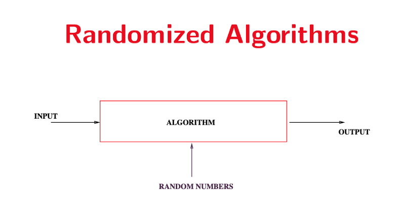
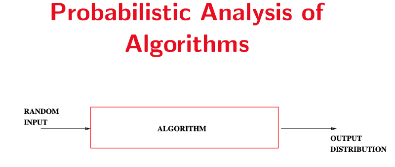
These algorithms are often trivial to come up with. But it is much more complex to analyze and prove the running time/correctness. It is worth noting that there is a difference between probabilistic analysis and analysis of randomized algorithms. In probabilistic analysis we give the algorithm an input assumed to be from a probability distribution. Whereas in the randomized algorithm we add a random number(s) to the input. The following images should show the distinction. Images are from Stanford lecture slides.
In this article, I will go through the contention resolution problem from Algorithm Design by Kleinberg and Tardos.
Contention Resolution
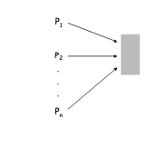
The problem is there are n processors that share a single database D and the time is divided into k discrete intervals. The database serves at most 1 processor at a time.
Goal: Divide the rounds among the n processors in an equitable fashion.
Keep in mind there is no communication between the processors of any sort to plan out when to access the database. If every processor keeps repeatedly trying to access D at the same time then the database will be locked out, serving 0 processors. Not ideal. By randomizing the sequence of access attempts from the processors we can “smooth out” the contention, avoiding lockouts.
Events
We need to specify some events and the probabilities associated with them.
Think about what is happening here, a processor i is trying to access D at time t. Let that be our first event.
E1 = A[i, t]: P[i] (process i) attempts to access D at round t
This event has a compliment, the process not attempting to access at round t.
E1^ = A[i, t]^: P[i] doesn’t attempt to access D at round t
Let A[i, t] have a probability of it occurring be p and since all individual probabilities in a sample space S = {E1, E1^} add up to 1, we have a probability of A[i,t]^ be 1-p.
Pr[A[i,t]] = p | Pr[A[i,t]^] = 1-p
After attempting to access the database, one of two things happens for process P[i]: it either succeeds or it doesn’t.
E2 = S[i,t]: P[i] succeeds in accessing D at round t
E2^ = S[i,t]^: P[i] doesn’t succeed in accessing D at round t
Success only happens when P[i] is attempting to access D and all other processes aren’t. This is an intersection of events E1 for all the processes.
S[i,t] = A[i,t] ∩ (∩j≠i A[j,t]^)
The probability of S[i,t] is, therefore, the probability of A[i,t] multiplied with the product of A[j,t]^ complement events.
Pr[S[i,t]] = Pr[A[i,t]] * ∏j≠i Pr[A[j,t]^] = p(1-p)^(n-1)
Remember derivatives? They equal 0 at minimums or maximums. Let f(p) = p(1-p)^(n-1) then the derivative of f(p) is
f’(p) = (1-p)^(n-1)- (n-1)p(1-p)^n-2
The obvious values that make this equation equal 0 are 0 and 1. When p = 0, none of the processes are attempting to access the database. When it equals 1 then all the processes are attempting at the same time. Both situations are ones we are not interested in. The only other value is when p = 1/n.
Set p = 1/n and we get
Pr[S[i,t]] = 1/n(1–1/n)^(n-1)
From calculus, there are two facts we will use.
- (1–1/n)^n converges monotonically from 1/4 up to 1/e
- (1–1/n)^n-1 converges monotonically from 1/2 down to 1/e
So we see there is an asymptotic bound we can use.
1/n(1–1/n)^(n-1) converges monotonically from (≤) 1/2 1/n down to (≥) 1/e1/n
1/en ≤ Pr[S[i,t]] ≤ 1/2n
The prior is asymptotically equal to O(1/n)
Another event, failures…
E3 = F[i,t]: denotes the “failure event” of P[i] not succeeding accesses to D in any rounds from 1 to t
That is equivalent to specifying the intersection of events, S[i,r]^ (no success) for r = 1…t
This eventually helps the probability of F[i,t] become a nice commutable math equation as the probability of the intersection of events is the product of the individual event probabilities.
Pr[F[i,t]] = Pr[⋂r=1.to.t (S[i,r]^)] = ∏r=1.to.t(Pr[S[i,r]^]) =
(1-p(1-p)^(n-1))^t
- Pr[S[i,t]] = p(1-p)^(n-1), S[i,t]^ = 1-Pr[S[i,t]]
Remember the calculus convergence properties we saw earlier? We use them here to get
Pr[F[i,t]] = (1-p(1-p)^(n-1))^t = (1–1/n(1–1/n)^(n-1))^t ≤ (1–1/en)^t
- p = 1/n because each of the n processors has an equal probability of attempting to access the database at time t
Now let us take a look at parameter t.
If we set t = ceiling(en) to make sure it is an integer, we get
Pr[F[i,t]] ≤ (1–1/en)^ceiling(en) ≤ (1–1/en)^en ≤ 1/e
This bound tells us that the probability of a process i not succeeding in its attempts from rounds 1 to ceiling(en) is upper-bounded by 1/e, independent of n.
Set t = ceiling(en)(cln(n)) then we have
Pr[F[i,t]] ≤ (1–1/en)^t ≤ ((1–1/en)^ceiling(en))^(cln(n)) ≤ (1/e)^cln(n) ≤ 1/n^c = n^-c
One last event… our goal is to have the processes succeed as many rounds as possible. In other words if, say,
E4 = F[t]: denotes the event of the protocol failing after t rounds then we would like to minimize t here to maximize the number of rounds it succeeds.
F[t] essentially occurs if and only if one of F[i,t] occurs, only takes one process failing to say the protocol has failed. This is therefore the union of events F[i,t] for processes i = 1…n.
F[t] = ⋃i=1.to.n(F[i,t])
Union Bound
The prior is hard to compute exactly because the events F[i,t] are not independent. The easy solution is bound to them as if they are all independent.
Given events E1, … En, we have Pr[⋃i=1.to.n(Ei)] ≤ ∑i=1.to.n(Pr[Ei])
Pr[F[t]] ≤ ∑i=1.to.n(Pr[F[i,t]])
Recall when t = ceiling(en)cln(n) gives an upper bound on Pr[F[i,t]] ≤ n^-c
Let c = 2 and we have Pr[F[t]] ≤ ∑i=1.to.n(n^(-2)) = n*n^(-2) = 1/n
What is the probability that all the processes succeed at accessing D at least once within the t = 2ceiling(en)ln(n) rounds?
Take the complement of F[t], F[t]^ and arrive at a probability
1–1/n.
Wrapping up
This was quite a lengthy analysis, and most analyses for randomized algorithms are. It is essentially a trade-off, as the algorithms are easier to design and understand than complex deterministic algorithms that are computationally heavy arriving at the correct solution. With randomized algorithms, we are willing to accept some small error with the luxury of efficiency.
Thank you for reading. I am new to the blogging game, so any feedback would be appreciated.