
By Bert Carremans
In this tutorial, I will explore some text mining techniques for sentiment analysis. We'll look at how to prepare textual data. After that we will try two different classifiers to infer the tweets' sentiment. We will tune the hyperparameters of both classifiers with grid search. Finally, we evaluate the performance on a set of metrics like precision, recall and the F1 score.
For this project, we'll be working with the Twitter US Airline Sentiment data set on Kaggle. It contains the tweet’s text and one variable with three possible sentiment values. Let's start by importing the packages and configuring some settings.
import numpy as np
import pandas as pd
pd.set_option('display.max_colwidth', -1)
from time import time
import re
import string
import os
import emoji
from pprint import pprint
import collections
import matplotlib.pyplot as plt
import seaborn as sns
sns.set(style="darkgrid")
sns.set(font_scale=1.3)
from sklearn.base import BaseEstimator, TransformerMixin
from sklearn.feature_extraction.text import CountVectorizer
from sklearn.feature_extraction.text import TfidfVectorizer
from sklearn.model_selection import GridSearchCV
from sklearn.model_selection import train_test_split
from sklearn.pipeline import Pipeline, FeatureUnion
from sklearn.metrics import classification_report
from sklearn.naive_bayes import MultinomialNB
from sklearn.linear_model import LogisticRegression
from sklearn.externals import joblib
import gensim
from nltk.corpus import stopwords
from nltk.stem import PorterStemmer
from nltk.tokenize import word_tokenize
import warnings
warnings.filterwarnings('ignore')
np.random.seed(37)
Loading the data
We read in the comma separated file we downloaded from the Kaggle Datasets. We shuffle the data frame in case the classes are sorted. Applying the reindex method on the permutation of the original indices is good for that. In this notebook, we will work with the text variable and the airline_sentiment variable.
df = pd.read_csv('../input/Tweets.csv')
df = df.reindex(np.random.permutation(df.index))
df = df[['text', 'airline_sentiment']]
Exploratory Data Analysis
Target variable
There are three class labels we will predict: negative, neutral or positive.
The class labels are imbalanced as we can see below in the chart. This is something that we should keep in mind during the model training phase. With the factorplot of the seaborn package, we can visualize the distribution of the target variable.
sns.factorplot(x="airline_sentiment", data=df, kind="count", size=6, aspect=1.5, palette="PuBuGn_d")
plt.show();
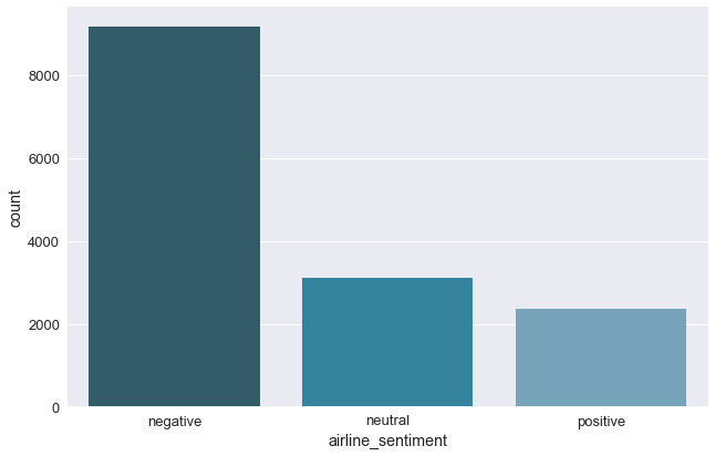 Imbalanced distribution of the target class labels
Input variable
To analyze the text variable we create a class TextCounts. In this class we compute some basic statistics on the text variable.
count_words: number of words in the tweetcount_mentions: referrals to other Twitter accounts start with a @count_hashtags: number of tag words, preceded by a #count_capital_words: number of uppercase words are sometimes used to “shout” and express (negative) emotionscount_excl_quest_marks: number of question or exclamation markscount_urls: number of links in the tweet, preceded by http(s)count_emojis: number of emoji, which might be a good sign of the sentiment
class TextCounts(BaseEstimator, TransformerMixin):

    def count_regex(self, pattern, tweet):
        return len(re.findall(pattern, tweet))

    def fit(self, X, y=None, **fit_params):
        # fit method is used when specific operations need to be done on the train data, but not on the test data
        return self

    def transform(self, X, **transform_params):
        count_words = X.apply(lambda x: self.count_regex(r'\w+', x))
        count_mentions = X.apply(lambda x: self.count_regex(r'@\w+', x))
        count_hashtags = X.apply(lambda x: self.count_regex(r'#\w+', x))
        count_capital_words = X.apply(lambda x: self.count_regex(r'\b[A-Z]{2,}\b', x))
        count_excl_quest_marks = X.apply(lambda x: self.count_regex(r'!|\?', x))
        count_urls = X.apply(lambda x: self.count_regex(r'http.?://[^\s]+[\s]?', x))
        # We will replace the emoji symbols with a description, which makes using a regex for counting easier
        # Moreover, it will result in having more words in the tweet
        count_emojis = X.apply(lambda x: emoji.demojize(x)).apply(lambda x: self.count_regex(r':[a-z_&]+:', x))

        df = pd.DataFrame({'count_words': count_words
                           , 'count_mentions': count_mentions
                           , 'count_hashtags': count_hashtags
                           , 'count_capital_words': count_capital_words
                           , 'count_excl_quest_marks': count_excl_quest_marks
                           , 'count_urls': count_urls
                           , 'count_emojis': count_emojis
                          })

        return df
tc = TextCounts()
df_eda = tc.fit_transform(df.text)
df_eda['airline_sentiment'] = df.airline_sentiment
It could be interesting to see how the TextStats variables relate to the class variable. So we write a function show_dist that provides descriptive statistics and a plot per target class.
def show_dist(df, col):
    print('Descriptive stats for {}'.format(col))
    print('-'*(len(col)+22))
    print(df.groupby('airline_sentiment')[col].describe())
    bins = np.arange(df[col].min(), df[col].max() + 1)
    g = sns.FacetGrid(df, col='airline_sentiment', size=5, hue='airline_sentiment', palette="PuBuGn_d")
    g = g.map(sns.distplot, col, kde=False, norm_hist=True, bins=bins)
    plt.show()
Below you can find the distribution of the number of words in a tweet per target class. For brevity, we will limit us to only this variable. The charts for all TextCounts variables are in the notebook on Github.
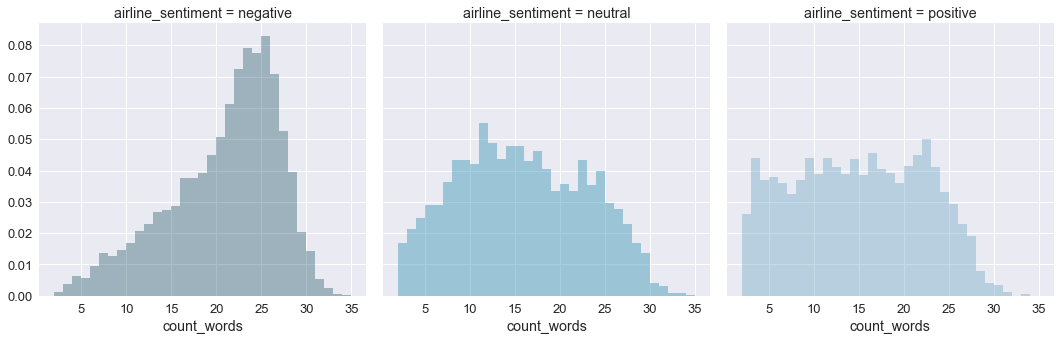
- The number of words used in the tweets is rather low. The largest number of words is 36 and there are even tweets with only 2 words. So we’ll have to be careful during data cleaning not to remove too many words. But the text processing will be faster. Negative tweets contain more words than neutral or positive tweets.
- All tweets have at least one mention. This is the result of extracting the tweets based on mentions in the Twitter data. There seems to be no difference in the number of mentions with regard to the sentiment.
- Most of the tweets do not contain hash tags. So this variable will not be retained during model training. Again, no difference in the number of hash tags with regard to the sentiment.
- Most of the tweets do not contain capitalized words and we do not see a difference in distribution between the sentiments.
- The positive tweets seem to be using a bit more exclamation or question marks.
- Most tweets do not contain a URL.
- Most tweets do not use emojis.
Text Cleaning
Before we start using the tweets’ text we need to clean it. We’ll do the this in the class CleanText. With this class we’ll perform the following actions:
- remove the mentions, as we want to generalize to tweets of other airline companies too.
- remove the hash tag sign (#) but not the actual tag as this may contain information
- set all words to lowercase
- remove all punctuations, including the question and exclamation marks
- remove the URLs as they do not contain useful information. We did not notice a difference in the number of URLs used between the sentiment classes
- make sure to convert the emojis into one word.
- remove digits
- remove stopwords
- apply the
PorterStemmerto keep the stem of the words
class CleanText(BaseEstimator, TransformerMixin):
    def remove_mentions(self, input_text):
        return re.sub(r'@\w+', '', input_text)

    def remove_urls(self, input_text):
        return re.sub(r'http.?://[^\s]+[\s]?', '', input_text)

    def emoji_oneword(self, input_text):
        # By compressing the underscore, the emoji is kept as one word
        return input_text.replace('_','')

    def remove_punctuation(self, input_text):
        # Make translation table
        punct = string.punctuation
        trantab = str.maketrans(punct, len(punct)*' ')  # Every punctuation symbol will be replaced by a space
        return input_text.translate(trantab)
    def remove_digits(self, input_text):
        return re.sub('\d+', '', input_text)

    def to_lower(self, input_text):
        return input_text.lower()

    def remove_stopwords(self, input_text):
        stopwords_list = stopwords.words('english')
        # Some words which might indicate a certain sentiment are kept via a whitelist
        whitelist = ["n't", "not", "no"]
        words = input_text.split()
        clean_words = [word for word in words if (word not in stopwords_list or word in whitelist) and len(word) > 1]
        return " ".join(clean_words)

    def stemming(self, input_text):
        porter = PorterStemmer()
        words = input_text.split()
        stemmed_words = [porter.stem(word) for word in words]
        return " ".join(stemmed_words)

    def fit(self, X, y=None, **fit_params):
        return self

    def transform(self, X, **transform_params):
        clean_X = X.apply(self.remove_mentions).apply(self.remove_urls).apply(self.emoji_oneword).apply(self.remove_punctuation).apply(self.remove_digits).apply(self.to_lower).apply(self.remove_stopwords).apply(self.stemming)
        return clean_X
To show how the cleaned text variable will look like, here’s a sample.
ct = CleanText()
sr_clean = ct.fit_transform(df.text)
sr_clean.sample(5)
glad rt bet bird wish flown south winter
point upc code check baggag tell luggag vacat day tri swimsuit
vx jfk la dirti plane not standard
tell mean work need estim time arriv pleas need laptop work thank
sure busi go els airlin travel name kathryn sotelo
One side-effect of text cleaning is that some rows do not have any words left in their text. For the CountVectorizer and TfIdfVectorizer this does not pose a problem. Yet, for the Word2Vec algorithm this causes an error. There are different strategies to deal with these missing values.
- Remove the complete row, but in a production environment this is not desirable.
- Impute the missing value with some placeholder text like [no_text]
- When applying Word2Vec: use the average of all vectors
Here we will impute with placeholder text.
empty_clean = sr_clean == ''
print('{} records have no words left after text cleaning'.format(sr_clean[empty_clean].count()))
sr_clean.loc[empty_clean] = '[no_text]'
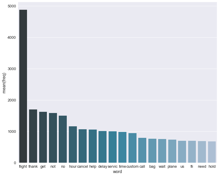
Now that we have the cleaned text of the tweets, we can have a look at what are the most frequent words. Below we’ll show the top 20 words. The most frequent word is “flight”.
cv = CountVectorizer()
bow = cv.fit_transform(sr_clean)
word_freq = dict(zip(cv.get_feature_names(), np.asarray(bow.sum(axis=0)).ravel()))
word_counter = collections.Counter(word_freq)
word_counter_df = pd.DataFrame(word_counter.most_common(20), columns = ['word', 'freq'])
fig, ax = plt.subplots(figsize=(12, 10))
sns.barplot(x="word", y="freq", data=word_counter_df, palette="PuBuGn_d", ax=ax)
plt.show();
Creating test data
To check the performance of the models we’ll need a test set. Evaluating on the train data would not be correct. You should not test on the same data used for training the model.
First, we combine the TextCounts variables with the CleanText variable. Initially, I made the mistake to execute TextCounts and CleanText in the GridSearchCV. This took too long as it applies these functions each run of the GridSearch. It suffices to run them only once.
df_model = df_eda
df_model['clean_text'] = sr_clean
df_model.columns.tolist()
So df_model now contains several variables. But our vectorizers (see below) will only need the clean_text variable. The TextCountsvariables can be added as such. To select columns, I wrote the class ColumnExtractor below.
class ColumnExtractor(TransformerMixin, BaseEstimator):
    def __init__(self, cols):
        self.cols = cols
    def transform(self, X, **transform_params):
        return X[self.cols]
    def fit(self, X, y=None, **fit_params):
        return self
X_train, X_test, y_train, y_test = train_test_split(df_model.drop('airline_sentiment', axis=1), df_model.airline_sentiment, test_size=0.1, random_state=37)
Hyperparameter tuning and cross-validation
As we will see below, the vectorizers and classifiers all have configurable parameters. To choose the best parameters, we need to test on a separate validation set. This validation set was not used during the training. Yet, using only one validation set may not produce reliable validation results. Due to chance, you might have a good model performance on the validation set. If you would split the data otherwise, you might end up with other results. To get a more accurate estimation, we perform cross-validation.
With cross-validation we split the data into a train and validation set many times. The evaluation metric is then averaged over the different folds. Luckily, GridSearchCV applies cross-validation out-of-the-box.
To find the best parameters for both a vectorizer and classifier, we create a Pipeline.
Evaluation metrics
By default GridSearchCV uses the default scorer to compute the best_score_. For both the MultiNomialNb and LogisticRegression this default scoring metric is accuracy.
In our function grid_vectwe additionally generate the classification_report on the test data. This provides some interesting metrics per target class. This might be more appropriate here. These metrics are the precision, recall and F1 score.
- Precision: Of all rows we predicted to be a certain class, how many did we correctly predict?
- Recall: Of all rows of a certain class, how many did we correctly predict?
- F1 score: Harmonic mean of Precision and Recall.
With the elements of the confusion matrix we can calculate Precision and Recall.
# Based on http://scikit-learn.org/stable/auto_examples/model_selection/grid_search_text_feature_extraction.html
def grid_vect(clf, parameters_clf, X_train, X_test, parameters_text=None, vect=None, is_w2v=False):

    textcountscols = ['count_capital_words','count_emojis','count_excl_quest_marks','count_hashtags'
                      ,'count_mentions','count_urls','count_words']

    if is_w2v:
        w2vcols = []
        for i in range(SIZE):
            w2vcols.append(i)
        features = FeatureUnion([('textcounts', ColumnExtractor(cols=textcountscols))
                                 , ('w2v', ColumnExtractor(cols=w2vcols))]
                                , n_jobs=-1)
    else:
        features = FeatureUnion([('textcounts', ColumnExtractor(cols=textcountscols))
                                 , ('pipe', Pipeline([('cleantext', ColumnExtractor(cols='clean_text')), ('vect', vect)]))]
                                , n_jobs=-1)

    pipeline = Pipeline([
        ('features', features)
        , ('clf', clf)
    ])

    # Join the parameters dictionaries together
    parameters = dict()
    if parameters_text:
        parameters.update(parameters_text)
    parameters.update(parameters_clf)
    # Make sure you have scikit-learn version 0.19 or higher to use multiple scoring metrics
    grid_search = GridSearchCV(pipeline, parameters, n_jobs=-1, verbose=1, cv=5)

    print("Performing grid search...")
    print("pipeline:", [name for name, _ in pipeline.steps])
    print("parameters:")
    pprint(parameters)
    t0 = time()
    grid_search.fit(X_train, y_train)
    print("done in %0.3fs" % (time() - t0))
    print()
    print("Best CV score: %0.3f" % grid_search.best_score_)
    print("Best parameters set:")
    best_parameters = grid_search.best_estimator_.get_params()
    for param_name in sorted(parameters.keys()):
        print("\t%s: %r" % (param_name, best_parameters[param_name]))

    print("Test score with best_estimator_: %0.3f" % grid_search.best_estimator_.score(X_test, y_test))
    print("\n")
    print("Classification Report Test Data")
    print(classification_report(y_test, grid_search.best_estimator_.predict(X_test)))

    return grid_search
Parameter grids for GridSearchCV
In the grid search, we will investigate the performance of the classifier. The set of parameters used to test the performance are specified below.
# Parameter grid settings for the vectorizers (Count and TFIDF)
parameters_vect = {
    'features__pipe__vect__max_df': (0.25, 0.5, 0.75),
    'features__pipe__vect__ngram_range': ((1, 1), (1, 2)),
    'features__pipe__vect__min_df': (1,2)
}

# Parameter grid settings for MultinomialNB
parameters_mnb = {
    'clf__alpha': (0.25, 0.5, 0.75)
}

# Parameter grid settings for LogisticRegression
parameters_logreg = {
    'clf__C': (0.25, 0.5, 1.0),
    'clf__penalty': ('l1', 'l2')
}
Classifiers
Here we will compare the performance of a MultinomialNBand LogisticRegression.
mnb = MultinomialNB()
logreg = LogisticRegression()
CountVectorizer
To use words in a classifier, we need to convert the words to numbers. Sklearn’s CountVectorizer takes all words in all tweets, assigns an ID and counts the frequency of the word per tweet. We then use this bag of words as input for a classifier. This bag of words is a sparse data set. This means that each record will have many zeroes for the words not occurring in the tweet.
countvect = CountVectorizer()
# MultinomialNB
best_mnb_countvect = grid_vect(mnb, parameters_mnb, X_train, X_test, parameters_text=parameters_vect, vect=countvect)
joblib.dump(best_mnb_countvect, '../output/best_mnb_countvect.pkl')
# LogisticRegression
best_logreg_countvect = grid_vect(logreg, parameters_logreg, X_train, X_test, parameters_text=parameters_vect, vect=countvect)
joblib.dump(best_logreg_countvect, '../output/best_logreg_countvect.pkl')
TF-IDF Vectorizer
One issue with CountVectorizer is that there might be words that occur frequently. These words might not have discriminatory information. Thus they can be removed. TF-IDF (term frequency — inverse document frequency)can be used to down-weight these frequent words.
tfidfvect = TfidfVectorizer()
# MultinomialNB
best_mnb_tfidf = grid_vect(mnb, parameters_mnb, X_train, X_test, parameters_text=parameters_vect, vect=tfidfvect)
joblib.dump(best_mnb_tfidf, '../output/best_mnb_tfidf.pkl')
# LogisticRegression
best_logreg_tfidf = grid_vect(logreg, parameters_mnb, X_train, X_test, parameters_text=parameters_vect, vect=tfidfvect)
joblib.dump(best_logreg_tfidf, '../output/best_logreg_tfidf.pkl')
Word2Vec
Another way of converting the words to numerical values is to use Word2Vec. Word2Vec maps each word in a multi-dimensional space. It does this by taking into account the context in which a word appears in the tweets. As a result, words that are similar are also close to each other in the multi-dimensional space.
The Word2Vec algorithm is part of the gensim package.
The Word2Vec algorithm uses lists of words as input. For that purpose, we use the word_tokenize method of the the nltk package.
SIZE = 50
X_train['clean_text_wordlist'] = X_train.clean_text.apply(lambda x : word_tokenize(x))
X_test['clean_text_wordlist'] = X_test.clean_text.apply(lambda x : word_tokenize(x))
model = gensim.models.Word2Vec(X_train.clean_text_wordlist
, min_count=1
, size=SIZE
, window=5
, workers=4)
model.most_similar('plane', topn=3)
The Word2Vec model provides a vocabulary of the words in all the tweets. For each word you also have its vector values. The number of vector values is equal to the chosen size. These are the dimensions on which each word is mapped in the multi-dimensional space. Words with an occurrence less than min_count are not kept in the vocabulary.
A side effect of the min_count parameter is that some tweets could have no vector values. This is would be the case when the word(s) in the tweet occur in less than min_count tweets. Due to the small corpus of tweets, there is a risk of this happening in our case. Thus we set the min_count value equal to 1.
The tweets can have a different number of vectors, depending on the number of words it contains. To use this output for modeling we will calculate the average of all vectors per tweet. As such we will have the same number (i.e. size) of input variables per tweet.
We do this with the function compute_avg_w2v_vector. In this function we also check whether the words in the tweet occur in the vocabulary of the Word2Vec model. If not, a list filled with 0.0 is returned. Else the average of the word vectors.
def compute_avg_w2v_vector(w2v_dict, tweet):
    list_of_word_vectors = [w2v_dict[w] for w in tweet if w in w2v_dict.vocab.keys()]

    if len(list_of_word_vectors) == 0:
        result = [0.0]*SIZE
    else:
        result = np.sum(list_of_word_vectors, axis=0) / len(list_of_word_vectors)

    return result
X_train_w2v = X_train['clean_text_wordlist'].apply(lambda x: compute_avg_w2v_vector(model.wv, x))
X_test_w2v = X_test['clean_text_wordlist'].apply(lambda x: compute_avg_w2v_vector(model.wv, x))
This gives us a Series with a vector of dimension equal to SIZE. Now we will split this vector and create a DataFrame with each vector value in a separate column. That way we can concatenate the Word2Vec variables to the other TextCounts variables. We need to reuse the index of X_train and X_test. Otherwise this will give issues (duplicates) in the concatenation later on.
X_train_w2v = pd.DataFrame(X_train_w2v.values.tolist(), index= X_train.index)
X_test_w2v = pd.DataFrame(X_test_w2v.values.tolist(), index= X_test.index)
# Concatenate with the TextCounts variables
X_train_w2v = pd.concat([X_train_w2v, X_train.drop(['clean_text', 'clean_text_wordlist'], axis=1)], axis=1)
X_test_w2v = pd.concat([X_test_w2v, X_test.drop(['clean_text', 'clean_text_wordlist'], axis=1)], axis=1)
We only consider LogisticRegression as we have negative values in the Word2Vec vectors. MultinomialNB assumes that the variables have a multinomial distribution. So they cannot contain negative values.
best_logreg_w2v = grid_vect(logreg, parameters_logreg, X_train_w2v, X_test_w2v, is_w2v=True)
joblib.dump(best_logreg_w2v, '../output/best_logreg_w2v.pkl')
Conclusion
- Both classifiers achieve the best results when using the features of the CountVectorizer
- Logistic Regression outperforms the Multinomial Naive Bayes classifier
- The best performance on the test set comes from the LogisticRegression with features from CountVectorizer.
Best parameters
- C value of 1
- L2 regularization
- max_df: 0.5 or maximum document frequency of 50%.
- min_df: 1 or the words need to appear in at least 2 tweets
- ngram_range: (1, 2), both single words as bi-grams are used
Evaluation metrics
- A test accuracy of 81,3%. This is better than a baseline performance of predicting the majority class (here a negative sentiment) for all observations. The baseline would give 63% accuracy.
- The Precision is rather high for all three classes. For instance, of all cases that we predict as negative, 80% is negative.
- The Recall for the neutral class is low. Of all neutral cases in our test data, we only predict 48% as being neutral.
Apply the best model on new tweets
For the fun, we will use the best model and apply it to some new tweets that contain @VirginAmerica. I selected 3 negative and 3 positive tweets by hand.
Thanks to the GridSearchCV, we now know what are the best hyperparameters. So now we can train the best model on all training data, including the test data that we split off before.
textcountscols = ['count_capital_words','count_emojis','count_excl_quest_marks','count_hashtags'
,'count_mentions','count_urls','count_words']
features = FeatureUnion([('textcounts', ColumnExtractor(cols=textcountscols))
, ('pipe', Pipeline([('cleantext', ColumnExtractor(cols='clean_text'))
, ('vect', CountVectorizer(max_df=0.5, min_df=1, ngram_range=(1,2)))]))]
, n_jobs=-1)
pipeline = Pipeline([
('features', features)
, ('clf', LogisticRegression(C=1.0, penalty='l2'))
])
best_model = pipeline.fit(df_model.drop('airline_sentiment', axis=1), df_model.airline_sentiment)
# Applying on new positive tweets
new_positive_tweets = pd.Series(["Thank you @VirginAmerica for you amazing customer support team on Tuesday 11/28 at @EWRairport and returning my lost bag in less than 24h! #efficiencyiskey #virginamerica"
,"Love flying with you guys ask these years. Sad that this will be the last trip ? @VirginAmerica #LuxuryTravel"
,"Wow @VirginAmerica main cabin select is the way to fly!! This plane is nice and clean & I have tons of legroom! Wahoo! NYC bound! ✈️"])
df_counts_pos = tc.transform(new_positive_tweets)
df_clean_pos = ct.transform(new_positive_tweets)
df_model_pos = df_counts_pos
df_model_pos['clean_text'] = df_clean_pos
best_model.predict(df_model_pos).tolist()
# Applying on new negative tweets
new_negative_tweets = pd.Series(["@VirginAmerica shocked my initially with the service, but then went on to shock me further with no response to what my complaint was. #unacceptable @Delta @richardbranson"
,"@VirginAmerica this morning I was forced to repack a suitcase w a medical device because it was barely overweight - wasn't even given an option to pay extra. My spouses suitcase then burst at the seam with the added device and had to be taped shut. Awful experience so far!"
,"Board airplane home. Computer issue. Get off plane, traverse airport to gate on opp side. Get on new plane hour later. Plane too heavy. 8 volunteers get off plane. Ohhh the adventure of travel ✈️ @VirginAmerica"])
df_counts_neg = tc.transform(new_negative_tweets)
df_clean_neg = ct.transform(new_negative_tweets)
df_model_neg = df_counts_neg
df_model_neg['clean_text'] = df_clean_neg
best_model.predict(df_model_neg).tolist()
The model classifies all tweets correctly. A larger test set should be used to assess the model’s performance. But on this small data set it does what we are aiming for. I hope you enjoyed reading this story. If you did, feel free to share it.