
By Rishit Dagli
In this article, I'll explain two important concepts in statistics: skewness and kurtosis. And don't worry – you won't need to know very much math to understand these concepts and learn how to apply them.
What are Density Curves?
Let's first talk a bit about density curves, as skewness and kurtosis are based on them. They're simply a way for us to represent a distribution. Let's see what I mean through an example.
Say that you need to record the heights of a lot of people. So your distribution has let's say 20 categories representing the range of the output (58-59 in, 59-60 in ... 78-79). You can plot a histogram representing these categories and the number of people whose height falls in each category.
 Histogram of height vs population
Well, you might do this for thousands of people, so you are not interested in the exact number – rather the percentage or probability of these categories.
I also explicitly mentioned that you have a rather large distribution since percentages are often useless for smaller distributions.
If you use percentages with smaller numbers I often refer to it as lying with statistics – it's a statement that is technically correct but creates the wrong impression in our minds.
Let me give you an example: a student is extremely excited and tells everyone in his class that he made a 100% improvement in his marks! But what he doesn't say is that his marks went from a 2/30 to 4/30 😂.
I hope you now clearly see the problem of using percentages with smaller numbers.
Coming back to density curves, when you are working with a large distribution you want to have more granular categories. So you make each category which was 1 inch wide now 2 categories each (\frac{1}{2}) inch wide. Maybe you want to get even more granular and start using (\frac{1}{4}) inch wide categories. Can you guess where I am going with this?
At a point, we get an infinite number of such categories with an infinitely small length. This allows us to create a curve from this histogram which we had earlier divided into discrete categories. See our density curve below drawn from the histogram.
 Probability density curve for our distribution
Why go through the effort?
Great question! As you may have guessed, I like to explain myself with examples, so let's look at another density curve to make it a bit easier for us to understand. Feel free to skip the curve equation at this stage if you have not worked with distributions before.
You can also follow along and create the graphs and visualizations in this article yourself through this Geogebra project (it runs in the browser).
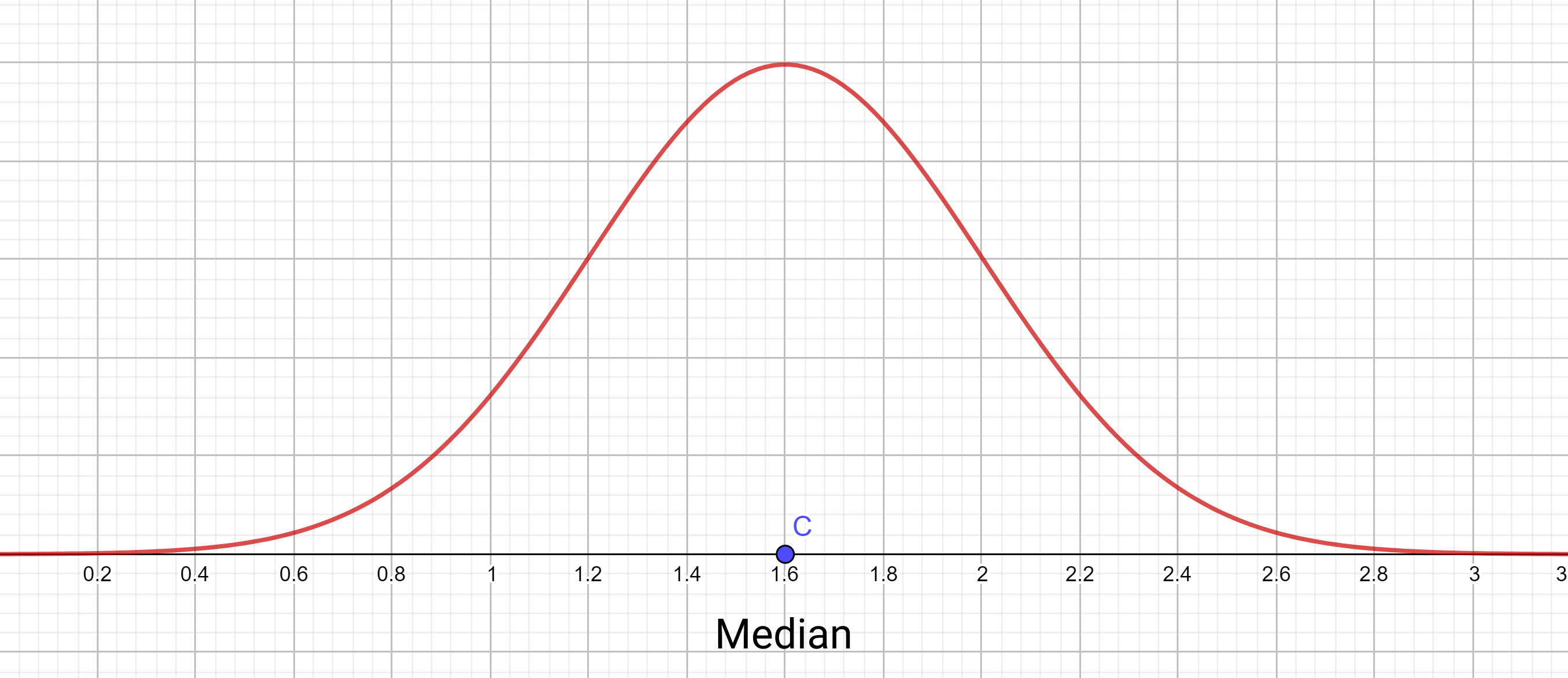
$$ f(x) = \frac{1}{0.4 \sqrt{2 \pi} } \cdot e^{-\frac{1}{2} (\frac{x - 1.6}{0.4})^2} $$

So now what if I ask you "What percent of my distribution is in the category 1 - 1.6?" Well, you just calculate the area under the curve between 1 and 1.6, like this:
$$ \int_{1}^{1.6} f(x) \,dx $$

It would also be relatively easy for you to answer similar questions from the density curve like: "What percent of the distribution is under 1.2?" or "What percent of the distribution is above 1.2?"
You can now probably see why the effort of making this making a density curve is worth it and how it allows you to make inferences easily 🚀.
Skewed Distributions
Let's now talk a bit about skewed distributions – that is, those that are not as pleasant and symmetric as the curves we saw earlier. We'll talk about this more intuitively using the ideas of mean and median.
From this density curve graph's image, try figuring out where the median of this distribution would be. Perhaps it was easy for you to figure out – the curve is symmetrical and you might have concluded that the median is 1.6 since it was symmetric about (x=1.6).
Another way to go about this would be to say that the median is the value where the area under the curve to the left of it it and the area under the curve to the right of it are equal.
We're talking about this idea since it allows us to also calculate the median for non-symmetric density curves.
As an example here, I show two very common skewed distributions and how the idea of equal areas we just discussed helps us find their medians. If we tried eyeballing our median, this is what we'd get since we want the areas on either side to be equal.
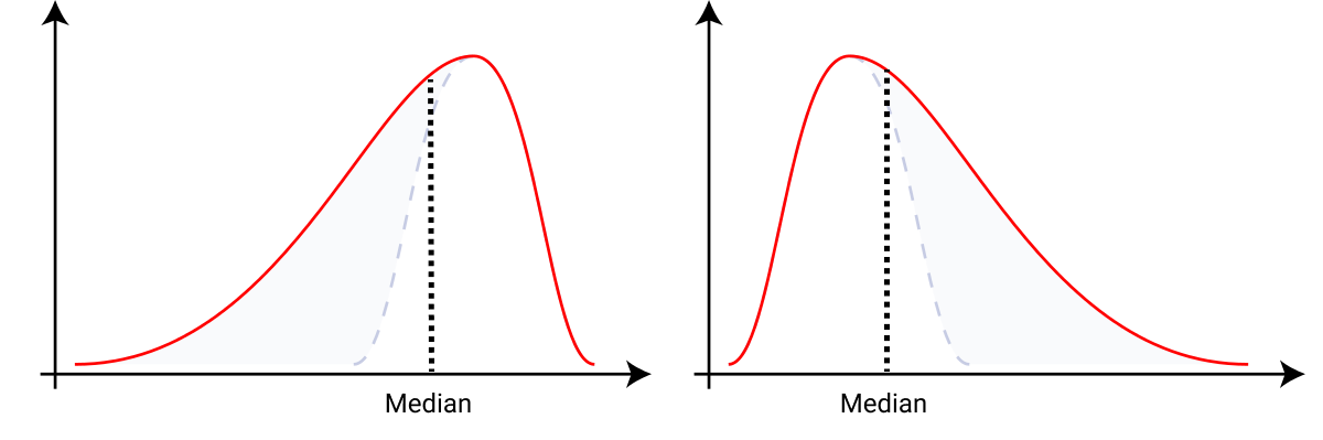 Eyeballing the median for skewed curves
You can also calculate the mean through these density curves. Maybe you've tried calculating the mean yourself already, but notice that if you use the general formula to calculate the mean:
$$ mean = \frac{\sum a_n}{n} $$
you might notice a flaw in it: we take into account the ( x ) values but we also have probabilities associated with these values too. And it just makes sense to factor that in too.
So we modify the way we calculate the mean by using weighted averages. We will now also have a term (w_n) representing the associated weights:
$$ mean = \frac{\sum{a_n \cdot w_n}}{n} $$
So, we will be using the idea we just discussed to calculate the mean from our density curve.
You can also more intuitively understand this as the point on the x-axis where you could place a fulcrum and balance the curve if it was a solid object. This idea should help you better understand finding the mean from our density curve.
But another really interesting way to look at this would be as the x-coordinate of the point on this curve where the rotational inertia would be zero.
You might have already figured out how we can locate the mean for symmetric curves: our median and mean lie at the same point, the point of symmetry.
We will be using the idea we just discussed, placing a fulcrum on the x-axis and balancing the curve, to eyeball out the mean for skewed graphs like the ones we saw earlier while calculating the median.
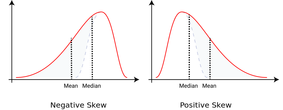
We will soon discuss the idea of skewness in greater detail. But at this stage, generally speaking, you can identify the direction where your curve is skewed. If the median is to the right of the mean, then it is negatively skewed. And if the mean is to the right of median, then it is positively skewed.
Later in this article, for simplicity's sake we'll also refer to the narrow part of these curves as a "tail".
What are Moments?
Before we talk more about skewness and kurtosis let's explore the idea of moments a bit. Later we'll use this concept to develop an idea for measuring skewness and kurtosis in our distribution.
We'll use a small dataset, [1, 2, 3, 3, 3, 6]. These numbers mean that you have points that are 1 unit away from the origin, 2 units away from the origin, and so on.
So, we care a lot about the distances from the origin in our dataset. We can represent the average distance from the origin in our data by writing:
$$ \frac{\sum a_n -0}{n} = \frac{\sum a_n}{n} $$
This is what we call our first moment. Calculating this for our sample dataset we get 3 but if we change our dataset and make all elements equal to 3,
$$ [1, 2, 3, 3, 3, 6] \rightarrow [3, 3, 3, 3, 3, 3] $$
you'll see that our first moment remains the same. Can we devise something to differentiate our two datasets that have equal first moments? (PS: It's the second moment.)
We will calculate the average sum of squared distances rather than the average sum of distances:
$$ \frac{\sum (a_n)^2}{n} $$
Our second moment for our original dataset is 11.33 and for our new dataset is 9. Notice that the magnitude of the second moment is larger for our original dataset than the new one. Also, we have a higher value for the second moment in the original dataset because it is spread out and has a greater average squared distance.
Essentially we are saying that we have a couple of values in our original dataset larger than the mean value, which, when squared, increases our second moment by a lot.
Here's an interesting way of thinking about moments – assume our distribution is mass, and then the first moment would be the center of the mass, and the second moment would be the rotational inertia.
You can also see that our second moment is highly dependent on our first moment. But we are interested in knowing the information the second moment can give us independently.
To do so we calculate the squared distances from the mean or the first moment rather than from the origin.
$$ \frac{\sum (a_n- \mu_{1}^{'})^2 }{n} $$
Did you notice that we also intuitively derived a formula for variance? Going forward you will see how we use the ideas we just talked about to measure skewness and kurtosis.
Intro to Skewness and Kurtosis?
Let's see how we can use the idea of moments we talked about earlier to figure out how we can measure skewness (which you already have some idea about) and kurtosis.
What is Skewness?
Let's take the idea of moments we talked about just now and try to calculate the third moment. As you might have guessed, we can calculate the cubes of our distances. But as we discussed above, we are more interested in seeing the additional information the third moment provides.
So we want to subtract the second moment from our third moment. Later, we will also refer to this factor as the adjustment to the moment. So our adjusted moment will look like this:
$$ skewness = \frac{\sum (a_n - \mu)^3 }{n \cdot \sigma ^3} $$
This adjusted moment is what we call skewness. It helps us measure the asymmetry in the data.
Perfectly symmetrical data would have a skewness value of 0. A negative skewness value implies that a distribution has its tail on the left side of the distribution, while a positive skewness value has its tail on the on the right side of the distribution.
 Positive skew and negative skew
At this stage, it might seem like calculating skewness would be pretty tough to do since in the formulas we use the population mean ( \mu ) and the population standard deviation ( \sigma ) which we wouldn't have access to while taking a sample.
Instead, you only have the sample mean and the sample standard deviation, so we will soon see how you can use these.
What is Kurtosis?
As you might have guessed, this time we will calculate our fourth moment or use the fourth power of our distances. And like we talked about earlier we are interested in seeing the additional information this provides so we will also subtract out the adjustment factor from it.
This is what we call kurtosis or a measure of whether our data has a lot of outliers or very few outliers. This will look like:
$$ kurtosis = \frac{\sum (a_n - \mu)^4 }{n \cdot \sigma ^4} $$
A better term for what's going on here is to figure out if the distribution is heavy-tailed or light-tailed. We can compare this to a normal distribution.
If you do a simple substitution you'll see that the kurtosis for normal distribution is 3. And since we are interested in comparing kurtosis to the normal distribution, often we use excess kurtosis which simply subtracts 3 from the above equation.
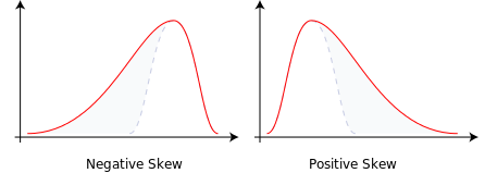
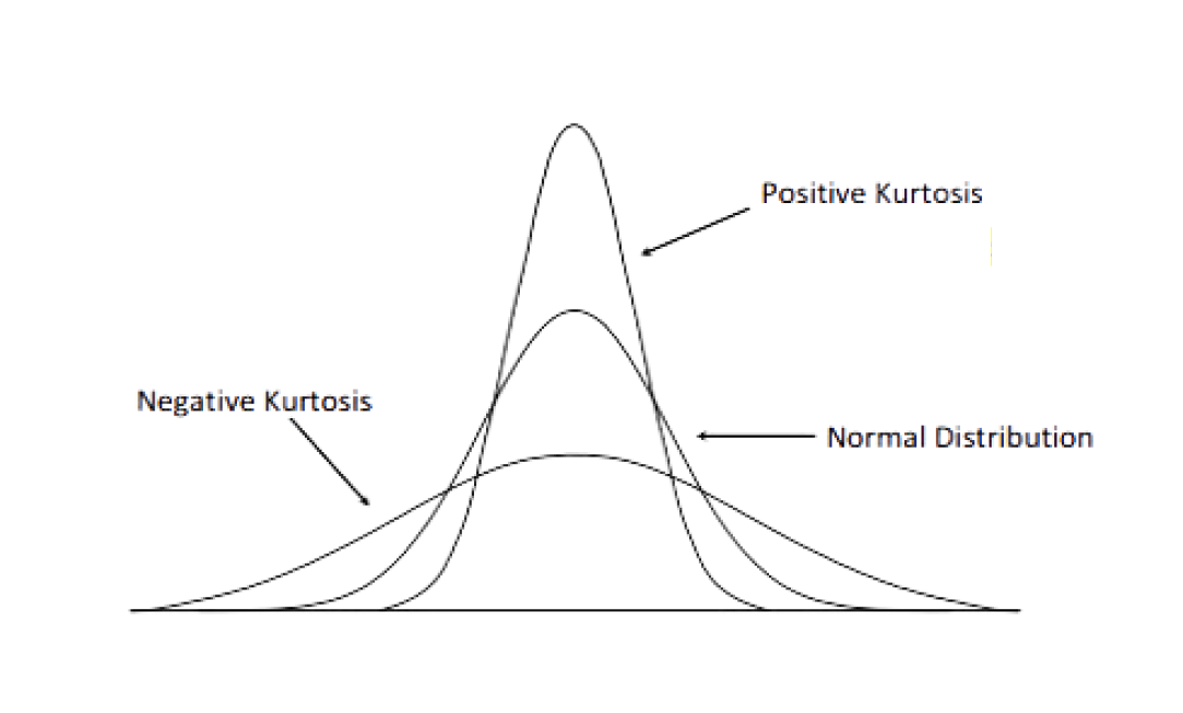 Positive and negative kurtosis (Adapted from Analytics Vidhya)
This is us essentially trying to force the kurtosis of our normal distribution to be 0 for easier comparison. So, if our distribution has positive kurtosis, it indicates a heavy-tailed distribution while negative kurtosis indicates a light-tailed distribution. Graphically, this would look something like the image above.
Sampling Adjustment
So, a problem with the equations we just built is that they have two terms in them, the distribution mean ( \mu ) and the distribution standard deviation ( \sigma ). But we are taking a sample of observations so we do not have the parameters for the whole distribution. We'd only have the sample mean and the sample standard deviation.
To keep this article focused, we will not be talking in detail about sampling adjustment terms since degrees of freedom is not in the scope of this article.
The idea is to use our sample mean ( \bar{x} ) and our sample standard deviation ( s ) to estimate these values for our distribution. We will also have to adjust our degree of freedom in these equations for it.
Don't worry if you don't understand this concept completely at this point. We can move on anyway. This leads to us modifying the equations we talked about earlier like so:
$$ skewness = \frac{\sum (a_n - \bar{x})^3 }{s^3} \cdot \frac{n}{(n-1)(n-2)} $$
$$ kurtosis = \frac{\sum (a_n - \bar{x})^4 }{s^4} \cdot \frac{n(n+1)}{(n-1)(n-2)(n-3)} - \frac{3(n-1)^2}{(n-2)(n-3)} $$
How to Implement this in Python
Finally, let's finish up by seeing how you can measure skewness and kurtosis in Python with an example. In case you want to follow along and try out the code, you can follow along with this Colab Notebook where we measure the skewness and kurtosis of a dataset.
It is pretty straightforward to implement this in Python with Scipy. It has methods to easily measure skewness and kurtosis for a distribution with pre-built methods.
The below code block shows how to measure skewness and kurtosis for the Boston housing dataset, but you could also use it for your own distributions.
from scipy.stats import skew
from scipy.stats import kurtosis

skew(data["MEDV"].dropna())
kurtosis(data["MEDV"].dropna())
Thank you for reading!
Thank you for sticking with me until the end. I hope you have learned a lot from this article.
I am excited to see if this article helped you better understand these two very important ideas. If you have any feedback or suggestions for me please feel free to reach out to me on Twitter.