
Over time, knowledge has been passed down in various forms. Before writing was invented in ancient Mesopotamia (modern-day Iraq), laws, history, myths, songs, and other information were all transferred from generation to generation orally. This was done either via instructions or storytelling (especially folktales and events that had happened over time).
But another common method of knowledge transfer is from teacher to student, whether formally or informally. We’ve seen this throughout time as well: the Bible recorded that Jesus had twelve disciples whom he taught daily from the start of his mission to his death. Socrates taught Plato. Plato went on to establish an academy in Athens, where he taught Aristotle for twenty years. Aristotle revolutionized science, logic, and politics. And the list goes on.
A 21st-century example of this is deep learning AI lineage. During the 20th-century AI winter, when we thought neural networks were a dead end, this teacher-student lineage kept the dream alive.
Geoffrey Hinton, regarded as the father of AI, ran a lab where he taught Yann LeCun, Ilya Sutskever, and others. Yann LeCun went on to invent the convolutional neural network (CNN), while Ilya Sutskever co-founded OpenAI before leaving for Safe Superintelligence Inc.
While the concept of knowledge transfer between humans is quite familiar, how about knowledge transfer from machine to machine? This is known as "model distillation."
In this article, I'm going to break down what model distillation is. We'll explore the techniques it uses, and I'll walk you through how to implement it from scratch using PyTorch.
By the end, you'll understand how to train smaller, more efficient models and how distillation compares to other compression techniques like quantization and pruning.
What We'll Cover
Prerequisites
To follow along, you should have the following:
A GitHub Repository: The complete implementation of the project is available here, and you should clone it to follow along.
Basic familiarity with Python and object-oriented programming concepts (for example, working with classes).
An overview of deep learning fundamentals. You should understand concepts like epochs, forward propagation, loss function, and so on.
PyTorch Basics: While I'll explain each code section for you, basic familiarity with PyTorch tensors and training loops will be helpful.
A development environment: You should have Python installed on your machine. I'll be using Visual Studio Code as my editor, but you can use any editor or IDE of your choice.
Hardware: For this project, we'll be using a relatively small dataset so a standard CPU will work well.
What is Model Distillation?
Model distillation (or knowledge distillation) is an approach that aims to pass on the learned behavior of a large, highly accurate model to a smaller, computationally efficient model that's better suited for practical deployment.
Distillation is a compression technique where a smaller model (known as the student) learns to mimic the output of a larger, more complex model (the teacher). The goal is for the student model to achieve a level of performance close to the teacher, but with significantly fewer parameters, making it more efficient for deployment. (Source)
Why is Model Distillation Necessary?
At the time of this writing, both closed-source and open-source models are trained on trillions of parameters. These are the internal configuration variables that models learn automatically from training data. This immense number of parameters makes it extremely difficult and expensive to run without proper funding. Models consume large amounts of energy and require expensive hardware.
With distillation, we can transfer the learnings of these frontier models to smaller, more efficient models, making them easier and cheaper to use.
Model Distillation Techniques
The distillation technique used depends on the knowledge that's being transferred. Some methods transfer only the final prediction. Others transfer internal representation, attention maps, reasoning steps, or even the entire behavior of the teacher model.
These are some of the techniques:
Response-Based Distillation
Originally introduced by Geoffrey Hinton in his paper Distilling the knowledge in a neural network, this is the classic teacher-to-student distillation. Before diving deep into how it works, there are a few concepts you need to understand about model training: hard labels and soft labels.
Hard labels deal strictly with fixed categorical targets. When a picture of a dog is fed into a model and it's asked to predict if it's a dog, cat, or horse, it predicts it's a dog, given the result as Dog(1), horse(0), and cat(0). There's no probability as to what percentage or features of the picture look like a cat or a horse.
But we also have soft labels, which deal with probability. When the same picture is fed to a model using soft labels, it can predict that the picture has a 0.85 probability of being a dog, a 0.10 probability of being a cat, and a 0.5 probability of being a horse.
In response-based distillation, instead of training the student model with hard labels, it also learns from the probability of the teacher model's output (soft labels). The student can learn that the picture is a dog, but it also learns that the picture also slightly resembles a cat and barely resembles a horse.
This additional information is called dark knowledge. It enables the smaller model to copy the behavior of a larger, more accurate teacher while maintaining high performance.
Some of the advantages of response-based distillation are that it's easy to implement, it's very stable, and it works well with image classification. But there are some drawbacks, the major one being that it ignores what happens inside the network.
That is, response base distillation only looks at the output layer (the probabilities), so the student has a "black-box" relationship with the teacher model. It learns what the teacher decides, but not how it comes to that conclusion. Using the previous example, it learns the probability of what feature is a dog, cat and horse but not the underlying principle or workings of how that conclusion was made.
Feature-Based Distillation
This technique transfers the internal feature representation of the larger model rather than transferring only the final output.
An easy way to think about this is to imagine that you're a student of a great math tutor. The tutor gives you a math problem and shows you their final result. You might eventually guess the right formula, but you're mostly just learning to memorize output.
But if the tutor requires you to look at their notebook and see their work, you're learning the tutor's exact thought process.
In feature-based distillation, during training, the student model is required to produce hidden layer activations that match those of the tutor using Mean Squared Error (MSE). With mean squared error, the student model isn't just rewarded for correctly guessing the final output. It's also penalised if its internal function system doesn't match that of the teacher model.
This method is heavily used in convolutional neural networks, vision transformers, object detection, and so on.
The drawbacks of this method are that since the student has to extract and store internal feature map of the teacher model at every training iteration, memory and power consumption can quickly escalate. This makes it very expensive to run.
Attention Distillation
In this approach, instead of the student model copying all the neurons, it observes where the larger model pays attention and copies those neurons.
In transformer models, which are models that try to make sense of a sentence instead of paying attention to individual words, attention maps indicate which input tokens or regions the model considers most important when making predictions. The student tries to reproduce those maps or the distribution of the teacher model. This shows the student where to "look" when trying to solve a problem.
The drawback of attention distillation is substantial overhead in both training time and hardware resource. This is because metrics like Mean Squared Error (MSE) and Kullback-Leibler (KL) divergence need to be calculated. These metrics act as a loss function that tells a model exactly how much it's prediction or internal representation differs from the teacher model. Making this calculation across massive attention tensors contribute significantly to resource consumption.
Self-Distillation
A model is also capable of training itself. This involves knowledge transfer from an earlier version to a later version. It can also involve the transfer of knowledge between different layers in the network.
An advantage of this is that the model can become better without necessarily growing in size, reducing the cost of using a larger model to train the student model.
How to Implement Knowledge Distillation in PyTorch.
To showcase how model distillation works in real time, we'll be training a teacher and then a student model using the MNIST dataset and classifier with PyTorch.
The dataset contains about 70,000 greyscale images of handwritten digits. We'll train the teacher, then freeze it while we train a student using hard labels and soft targets from the teacher.
Note that the MNIST dataset is a relatively small dataset, so our distillation gains might not be much. But this project showcases the distillation workflow, and it will give you a good background to run larger datasets.
To run this project, you'll need the following Python packages:
| Package | Purpose |
|---|---|
torch |
The core deep learning framework we'll use to build and train neural networks. |
torchvision |
Provides datasets like MNIST and image utilities. |
numpy |
Numerical computations and array operations. |
matplotlib |
Plotting graphs and visualizing the visual images/results. |
tqdm |
Displays progress bars during training. |
For this project, I'll be working with the Visual Studio Code editor, but you can use any other code editor of your choice.
This is our project structure. I'll be explaining the folders and files below alongside the code for our project.
knowledge-distillation/
│
├── data/
│
├── models.py
│
├── engine.py
│
├── losses.py
│
├── train_teacher.py
│
├── train_student.py
│
├── train_distilled_student.py
│
├── evaluate.py
│
├── visualize.py
│
├── utils.py
│
├── plots.py
│
├── requirements.txt
│
└── README.md
First in our folder structure is our data folder. This contains our MNIST dataset.
Our models.py file defines the architecture of every neural network used in the project. It contains the teacher network class and student network class. Each class defines layers, forward propagation, and how data flow through the network.
import torch
import torch.nn as nn
import torch.nn.functional as F

class TeacherNet(nn.Module):

    def __init__(self):
        super().__init__()

        self.flatten = nn.Flatten()

        self.fc1 = nn.Linear(28 * 28, 1024)
        self.fc2 = nn.Linear(1024, 512)
        self.fc3 = nn.Linear(512, 256)
        self.fc4 = nn.Linear(256, 128)
        self.fc5 = nn.Linear(128, 10)

    def forward(self, x):

        x = self.flatten(x)

        x = F.relu(self.fc1(x))
        x = F.relu(self.fc2(x))
        x = F.relu(self.fc3(x))
        x = F.relu(self.fc4(x))

        logits = self.fc5(x)

        return logits


class StudentNet(nn.Module):
    """
    Smaller neural network (Student)
    """

    def __init__(self):
        super().__init__()

        self.flatten = nn.Flatten()

        self.fc1 = nn.Linear(28 * 28, 128)
        self.fc2 = nn.Linear(128, 10)

    def forward(self, x):

        x = self.flatten(x)

        x = F.relu(self.fc1(x))

        logits = self.fc2(x)

        return logits
The utils.py file prepares the dataset and answers the question, "Where does the dataset come from?" Here, we download the MNIST dataset, normalize the images, and create our training and testing loader.
from torchvision import datasets, transforms
from torch.utils.data import DataLoader


def get_dataloaders(batch_size=64):
    """
    Downloads MNIST (if needed) and returns
    training and testing DataLoaders.
    """

    transform = transforms.ToTensor()

    train_dataset = datasets.MNIST(
        root="data",
        train=True,
        download=True,
        transform=transform
    )

    test_dataset = datasets.MNIST(
        root="data",
        train=False,
        download=True,
        transform=transform
    )

    train_loader = DataLoader(
        train_dataset,
        batch_size=batch_size,
        shuffle=True
    )

    test_loader = DataLoader(
        test_dataset,
        batch_size=batch_size,
        shuffle=False
    )

    return train_loader, test_loader
The engine.py file contains the reusable learning algorithm and helps with how training happens. It receives the model.py code and trains it.
import torch
from tqdm import tqdm


def train_one_epoch(
    model,
    dataloader,
    criterion,
    optimizer,
    device,
):
    model.train()

    running_loss = 0

    progress = tqdm(dataloader)

    for images, labels in progress:

        images = images.to(device)
        labels = labels.to(device)

        optimizer.zero_grad()

        outputs = model(images)

        loss = criterion(outputs, labels)

        loss.backward()

        optimizer.step()

        running_loss += loss.item()

        progress.set_description(
            f"Loss {loss.item():.4f}"
        )

    return running_loss / len(dataloader)


def evaluate(model, dataloader, device):

    model.eval()

    correct = 0
    total = 0

    with torch.no_grad():

        for images, labels in dataloader:

            images = images.to(device)
            labels = labels.to(device)

            outputs = model(images)

            _, predicted = torch.max(outputs, dim=1)

            total += labels.size(0)

            correct += (predicted == labels).sum().item()

    accuracy = 100 * correct / total

    return accuracy


def predict(model, images, device):

    model.eval()

    with torch.no_grad():

        images = images.to(device)

        outputs = model(images)

        _, predictions = torch.max(outputs, dim=1)

    return predictions

def train_distillation_epoch(
    teacher,
    student,
    dataloader,
    optimizer,
    device,
    loss_fn,
    temperature=4.0,
    alpha=0.5,
):
    """
    Train the student using a frozen teacher.
    """

    teacher.eval()
    student.train()

    running_loss = 0

    progress = tqdm(dataloader)

    for images, labels in progress:

        images = images.to(device)
        labels = labels.to(device)

        optimizer.zero_grad()

        # Teacher predictions (NO gradients)
        with torch.no_grad():
            teacher_logits = teacher(images)

        # Student predictions
        student_logits = student(images)

        # Combined loss
        loss = loss_fn(
            student_logits=student_logits,
            teacher_logits=teacher_logits,
            labels=labels,
            temperature=temperature,
            alpha=alpha,
        )

        loss.backward()

        optimizer.step()

        running_loss += loss.item()

        progress.set_description(
            f"Distill Loss {loss.item():.4f}"
        )

    return running_loss / len(dataloader)
The losses.py file defines how the model measures its mistake. Since a neural network learns by minimizing loss, for baseline visualize used CrossEntropyLoss, and for knowledge distillation, we introduced distillation_loss().
Inside this file, we combined hard labels and soft targets using cross entropy and k1 divergence. This is where Geoffrey Hinton's algorithm lives.
import torch
import torch.nn as nn
import torch.nn.functional as F

cross_entropy = nn.CrossEntropyLoss()


def distillation_loss(
    student_logits,
    teacher_logits,
    labels,
    temperature=4.0,
    alpha=0.5,
):
    """
    Geoffrey Hinton's Knowledge Distillation Loss

    Parameters
    ----------
    student_logits : output from student model
    teacher_logits : output from teacher model
    labels         : ground-truth labels
    temperature    : controls softness of probability distribution
    alpha          : weight between hard and soft losses
    """

    # Hard Label Loss
    hard_loss = cross_entropy(student_logits, labels)

    # Teacher Soft Targets
    teacher_probs = F.softmax(
        teacher_logits / temperature,
        dim=1
    )

    # Student Soft Predictions
    student_log_probs = F.log_softmax(
        student_logits / temperature,
        dim=1
    )

    # KL Divergence
    soft_loss = F.kl_div(
        student_log_probs,
        teacher_probs,
        reduction="batchmean"
    )

    # Final Distillation Loss
    loss = (
        alpha * hard_loss
        +
        (1 - alpha)
        * (temperature ** 2)
        * soft_loss
    )

    return loss
The train_teacher.py file is to train the teacher network. After running this for the first time, we don't train the teacher again.
import torch
import torch.optim as optim

from models import TeacherNet
from utils import get_dataloaders
from engine import train_one_epoch, evaluate
from losses import cross_entropy

device = torch.device(
    "cuda" if torch.cuda.is_available() else "cpu"
)

train_loader, test_loader = get_dataloaders()

teacher = TeacherNet().to(device)

optimizer = optim.Adam(
    teacher.parameters(),
    lr=0.001,
)

epochs = 10

for epoch in range(epochs):

    loss = train_one_epoch(
        teacher,
        train_loader,
        cross_entropy,
        optimizer,
        device,
    )

    accuracy = evaluate(
        teacher,
        test_loader,
        device,
    )

    print(
        f"Epoch {epoch+1}/{epochs}"
        f" | Loss: {loss:.4f}"
        f" | Accuracy: {accuracy:.2f}%"
    )

torch.save(
    teacher.state_dict(),
    "teacher.pth",
)

print("\nTeacher saved successfully.")
The train_student.py file is where we train the student. It's identical to that of the train_teacher except it's a smaller network and no teacher guidance is implemented here. This gives the baseline accuracy of how the student will perform without the teacher.
import torch
import torch.optim as optim

from models import StudentNet
from utils import get_dataloaders
from engine import train_one_epoch, evaluate
from losses import cross_entropy

device = torch.device(
    "cuda" if torch.cuda.is_available() else "cpu"
)

train_loader, test_loader = get_dataloaders()

student = StudentNet().to(device)

optimizer = optim.Adam(
    student.parameters(),
    lr=0.001,
)

epochs = 10

for epoch in range(epochs):

    loss = train_one_epoch(
        student,
        train_loader,
        cross_entropy,
        optimizer,
        device,
    )

    accuracy = evaluate(
        student,
        test_loader,
        device,
    )

    print(
        f"Epoch {epoch+1}/{epochs}"
        f" | Loss: {loss:.4f}"
        f" | Accuracy: {accuracy:.2f}%"
    )

torch.save(
    student.state_dict(),
    "student_baseline.pth",
)

print("\nBaseline student saved.")
The train_distilled_student.py is the heart of this code. In this file, we teach the student using both labels and the teacher's knowledge. Here, we implement response-based knowledge distillation.
import torch
import torch.optim as optim

from models import TeacherNet, StudentNet
from utils import get_dataloaders
from engine import (
    train_distillation_epoch,
    evaluate,
)
from losses import distillation_loss

device = torch.device(
    "cuda" if torch.cuda.is_available() else "cpu"
)

train_loader, test_loader = get_dataloaders()

# Load Teacher
teacher = TeacherNet().to(device)
teacher.load_state_dict(
    torch.load(
        "teacher.pth",
        map_location=device,
    )
)

teacher.eval()

# Student
student = StudentNet().to(device)

optimizer = optim.Adam(
    student.parameters(),
    lr=0.001,
)

epochs = 10

for epoch in range(epochs):

    loss = train_distillation_epoch(
        teacher,
        student,
        train_loader,
        optimizer,
        device,
        distillation_loss,
        temperature=3,
        alpha=0.7,
    )

    accuracy = evaluate(
        student,
        test_loader,
        device,
    )

    print(
        f"Epoch {epoch+1}/{epochs}"
        f" | Loss: {loss:.4f}"
        f" | Accuracy: {accuracy:.2f}%"
    )

torch.save(
    student.state_dict(),
    "student_distilled.pth",
)

print("\nDistilled student saved.")
The evaluate.py measures how well a trained model performs. Here, we simply load the model, load test data, predict, and compute the accuracy.
import torch

from models import TeacherNet
from utils import get_dataloaders
from engine import evaluate

device = torch.device(
    "cuda" if torch.cuda.is_available() else "cpu"
)

_, test_loader = get_dataloaders()

teacher = TeacherNet().to(device)

teacher.load_state_dict(
    torch.load(
        "teacher.pth",
        map_location=device,
    )
)

accuracy = evaluate(
    teacher,
    test_loader,
    device,
)

print(
    f"Teacher Accuracy: {accuracy:.2f}%"
)
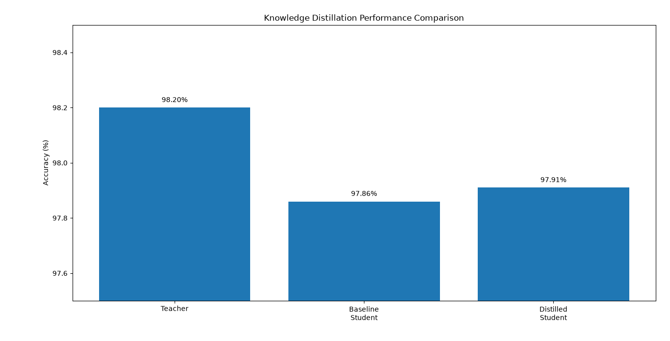
The visualize.py file is to present our findings visually. We use the Python package matplotlib to visualise the results of our teacher, baseline student, and distilled student.
import matplotlib.pyplot as plt

models = [
    "Teacher",
    "Baseline\nStudent",
    "Distilled\nStudent"
]

accuracy = [98.20, 97.86, 97.91]

plt.figure(figsize=(7,5))
plt.bar(models, accuracy)

plt.title("Knowledge Distillation Performance Comparison")
plt.ylabel("Accuracy (%)")

for i, v in enumerate(accuracy):
    plt.text(i, v + 0.02, f"{v:.2f}%", ha="center")

plt.ylim(97.5, 98.5)

plt.tight_layout()
plt.savefig("accuracy_comparison.png", dpi=300)
plt.show()
You can see the entire workflow of our program below so you understand how everything comes together:
                       utils.py
                          │
                 Load MNIST Dataset
                          │
                          ▼
                     models.py
             TeacherNet / StudentNet
                          │
                          ▼
                     losses.py
  Cross Entropy + Distillation Loss Function
                          │
                          ▼
                     engine.py
    Generic Training and Evaluation Functions
             ┌────────────┼────────────┐
             │            │            │
             ▼            ▼            ▼
  train_teacher.py  train_student.py  distilled_student.py
             │            │            │
             ▼            ▼            ▼
   teacher.pth  student_baseline.pth  distilled.pth
                          │
                          ▼
                     evaluate.py
              Compute Final Accuracy
                          │
                          ▼
                    visualize.py
     Generate Charts and Experimental Figures
How to Evaluate the Results
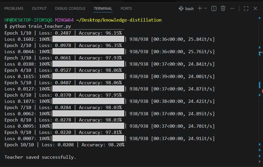
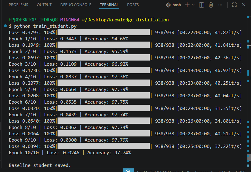
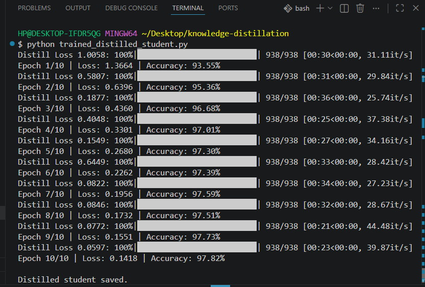
Now, let's check and evaluate our results. These are screenshots from running ten epochs for each of the networks: the teacher, student, and distilled student network.
Teacher Network: After 10 complete cycles, we attained an accuracy of 98.20%.
Student Network: After 10 complete cycles, we attained an accuracy of 97.74%. This is a pretty good performance for a smaller network without the teacher model.
Distilled Student Network: After 10 complete cycle, we attained an accuracy of 98.20%. We had an improvement from 97.74% achieved without the teacher's model knowledge.
Check out the chart below that shows how each model performed:
Other Approaches for Reducing Model Size
Now that we've seen what model distillation is with real-world code examples. Let's look at other approaches that developers are taking to reduce the size of large language models to save on latency, memory footprints, and compute cost and how they differ from distillation.
We have three other major approaches for this:
Quantization
Quantization achieves efficiency by strictly reducing the bit-width of the underlying data types used to store numerical weight and activations of the neural network. It targets the memory bandwidth bottleneck rather than the model architecture.
In simple terms, quantization can change a 32-bit number to 8-bit numbers, which saves about 75% of the file size.
A real-world example of how quantization differs from distillation is trying to save resources like ink and paper when printing a textbook. Distillation summarizes the textbook, while quantization prints the exact thing but uses a lower-resolution font to save ink and paper.
Pruning
Pruning operates on the principle that large language models often have too many redundant and low-impact parameters on the network. By removing weak connections, models can become smaller and faster.
For the textbook analogy, the pruning process is like going through the textbook and ripping off pages or chapters that you feel aren't needed.
Low-Rank Factorization
This is a mathematical process that uses linear algebra to simplify the matrix multiplication that dominates the deep learning architecture.
With the textbook example, this process involves rewriting complex sentences into simpler, shorter formulas that mean the same thing.
Choosing which method to use depends on the bottleneck you're trying to solve. Quantization generally works well for memory challenges, while pruning and distillation are designed to reduce computation time.
Conclusion
Knowledge transfer is as fundamental to artificial intelligence as it is to human history. Just as Aristotle built upon the teachings of Plato, today's efficient, deployable neural networks rely on the foundational "dark knowledge" extracted from massive, compute-heavy teacher models.
While training trillion-parameter frontier models requires immense hardware and financial resources, knowledge distillation ensures that the practical benefits of these advancements aren't locked behind massive computational bottlenecks.
As we demonstrated with the PyTorch MNIST experiment, even a simple response-based distillation can help a smaller network punch above its weight class by learning from the soft probabilities of a larger teacher.
When combined with other optimization techniques like quantization and pruning, distillation provides a clear pathway for deploying highly capable AI on edge devices, mobile phones, and consumer-grade hardware.
Thank you for reading! Please check out my YouTube channel, where I post videos on AI-related content.
References:
What does it mean to distill a machine learning model or LLM?
AI Insights: Model Distillation from the Department for Science, Innovation and Technology
Model distillation for LLMs: A practical guide to smaller, faster AI
Distilling knowledge in a neural network by Geoffrey Hinton


