

Have you ever performed some task without really thinking about the process involved? For example, making coffee, tying your shoes, or walking through your neighborhood.
In these types of activities, you've done these things so many times that you've mastered the process. You can be thinking about something unrelated, yet you perform these activities all the same. This phenomenon is called procedural memory in psychology.
We have this kind of thing with machine learning models as well, but it's not as positive as it is with humans. This is known as overfitting in machine learning.
What is Overfitting?
In overfitting, a model becomes so good at our training data that it has mastered every pattern, including noise. This makes the model perform well with training data but poorly with test or validation data.
The illustration below depicts how an optimal model fits into the data compared to overfitting.
In the graph, we have our features on the x-axis. In datasets, features are data that can be used to predict an outcome. The output variable is the outcome based on those features. The blue dots represent the data points where the features determine output variables.
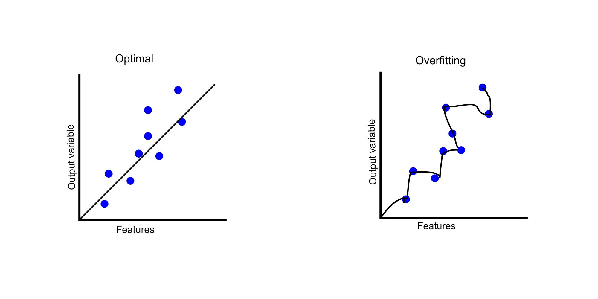
In the optimal graph, our model tries to find the generalized trend. But in our overfitted chart, the model tries to master each data point, resulting in an asymmetrical curve.
An example of a case study would be to predict if a customer would default on a bank loan. Assuming we have a dataset of 100,000 customers containing features such as demographics, income, loan amount, credit history, employment record, and default status, we split our data into training and test data.
Our training dataset contains 80,000 customers, while our test dataset contains 20,000 customers. In the training the dataset, we observe that our model has a 97% accuracy, but in prediction, we only get 50% accuracy. This shows that we have an overfitting problem.
Can you tell why overfitting is a problem? Yes! It produces an incorrect prediction. It is the purpose of machine learning models to make predictions to help business decision-making. We waste time and resources when our model makes incorrect predictions.
Imagine predicting that a customer will pay back a loan, and the customer defaults. Not just one customer but thousands of customers. This can cause a crisis for any financial institution.
Causes of Overfitting
Noisy data
Noise in data often appears as errors, fluctuations, or outliers in the data. This can be caused by data entry errors, data aging, data transmission errors, and so on.
Too much noise in data can cause the model to think these are valid data points. Fitting the noise pattern in the training dataset will cause poor performance on the new dataset.
For example, let's say that we are building a machine-learning model to classify images of cats and dogs. But some of the images in the dataset are blurry or poorly lit. While the model may perform well on the training data, it might struggle on the test data since it must have mastered some pattern with the blurry images in the dataset.
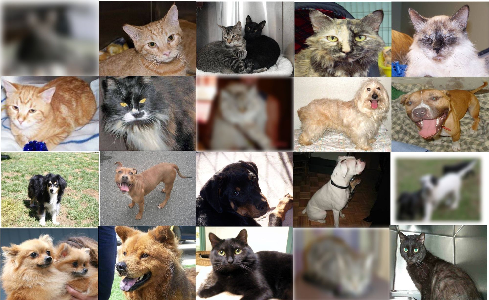
In the picture above, you can see that we have some blurry images that cannot be labelled if they are cat or dog. In these instances, the model could also learn these patterns alongside relevant features. Removing these images can reduce overfitting.
Insufficient training data
There will be fewer patterns and noises to analyze if we don't have sufficient training data. This means that the machine can only learn a little about our data.
Using our previous example, if our training data contains fewer images of dogs but many more of cats, the model learns so much about cats that when we feed the system an image of a dog, it will likely give a wrong output.
Overly complex model
In a complex model, there are many parameters capable of capturing patterns and relationships in training data. As a result, our model makes a more accurate prediction.
But this can pose a problem, since the model can start capturing noise, fluctuations, or outliers. Let's look at a decision tree model, how it works, and how overfitting can happen when it becomes too complex.
A decision tree model works by repeatedly breaking down data into significant features, making each point a node. This creates a tree like structure.
To make a prediction, it starts from the root node and follow the branches down, breaking and fitting every feature until it gets to the leaf node. The prediction is then made based on the value associated with the leaf node.
Let's look at a simple tree diagram of how a decision tree can predict if a customer is likely to default on loan base on certain features.
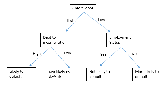 Tree diagram showing whether a customer is likely to default on a loan
This model starts by creating a parent node which is credit score. Depending on whether the credit score for the applicant is high or low, it goes down to the next node, which is either debt to income ratio or employment status. Then it makes the final prediction as to whether the customer is likely to default or not.
A decision tree can become overly complex when it creates too many nodes, making it too detailed or specific to the training data.
Let's see a sample machine learning program that predicts whether a customer will default a loan or not using decision tree model. For specificity, I wont be showing the cleaning process and visualization. I'll just lay emphasis on the required functions and how overfitting can happen with decision tree model.
The link to the complete repository containing cleaning and visualization can be found here, and you can get the dataset here.
import pandas as pd
import numpy as np
import matplotlib.pyplot as plt
import seaborn as sns
from sklearn.metrics import accuracy_score
from sklearn.model_selection import train_test_split
from sklearn.preprocessing import LabelEncoder
from sklearn import tree
from sklearn import metrics
from sklearn.tree import DecisionTreeClassifier

%matplotlib inline

#Importing our libraries
train = pd.read_csv('/content/train.csv')
test = pd.read_csv('/content/test.csv')

#Combine both training and test data
df = pd.concat([train, test], axis=0)
df.head()

#View dataset
train.head()

# Copy require features to a variable df_
df_ = train[['Gender',
'Married',
'Education',
'Self_Employed',
'Dependents',
'ApplicantIncome',
'CoapplicantIncome',
'LoanAmount',
'Loan_Amount_Term',
'Property_Area',
'Credit_History']]

### Duplicate a copy of df into X
X = df_.copy()

### label encode for Y
y = train['Loan_Status'].map({'N':0,'Y':1}).astype(int)

### train-test split
X_train, X_test, y_train, y_test = train_test_split(X, y, test_size=0.2, random_state=42)

# train
clf = DecisionTreeClassifier() #change model here
clf.fit(X_train, y_train)

# predict
predictions_clf = clf.predict(X_test)

#Print Accuracy
print('Model Accuracy:', accuracy_score(predictions_clf, y_test))
To understand this better, I'll explain what each module does:
import pandas as pd
import numpy as np
import matplotlib.pyplot as plt
import seaborn as sns
from sklearn.metrics import accuracy_score
from sklearn.model_selection import train_test_split
from sklearn.preprocessing import LabelEncoder
from sklearn import tree
from sklearn import metrics
from sklearn.tree import DecisionTreeClassifier
The first block is the import section. This is where we import all our dependencies.
- Numpy is a Python library used for scientific computing.
- Pandas is a library for data analysis and manipulation.
- Matplotlib and Seaborn are for statistical data visualization.
Accuracy_scoreis a function to calculate the accuracy of our model.train_test_splitis used to split our dataset into training and test data.- The
LabelEncoderencodes categorical variables into numeric variables. treeis for building a decision tree classifier.metricshelps us evaluate our models.
#Importing our dataset
train = pd.read_csv('/content/train.csv')
test = pd.read_csv('/content/test.csv')
This module imports our datasets. Our train and test datasets have been downloaded from the public repository, so we import them separately.
#Combine both training and test data
df = pd.concat([train, test], axis=0)
df.head()
To work with both datasets, we need to combine them into one dataset. The concat function combines both datasets. We use df.head() to visualize the dataset which is shown below.
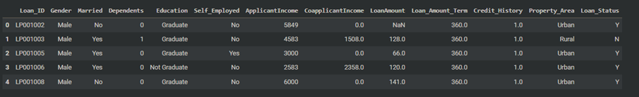 Screenshot of our dataset
# Copy require features to a variable df_
df_ = train[['Gender',
'Married',
'Education',
'Self_Employed',
'Dependents',
'ApplicantIncome',
'CoapplicantIncome',
'LoanAmount',
'Loan_Amount_Term',
'Property_Area',
'Credit_History']]

### Duplicate a copy of df into X
X = df_.copy()
To start working with our features, we created a variable df_ to store all the features needed for prediction. We duplicated this into the variable X to create a copy to work with.
### label encode for Y
y = train['Loan_Status'].map({'N':0,'Y':1}).astype(int)
To work with our outcome variable, we needed to convert it from a categorical value to an integer value. This also makes it easy for our model to understand. All values of N were converted to 0, while Y was converted to 1.
### train-test split
X_train, X_test, y_train, y_test = train_test_split(X, y, test_size=0.2, random_state=42)
We use our train_test_split to split our data into training and test data. The test_size = 0.2 means we are using 20% of the data for testing and 80% for training.
# train
clf = DecisionTreeClassifier()
clf.fit(X_train, y_train)
We assigned DecisionTreeClassifier() to the variable clf, which we'll use to train and fit our data. DecisionTreeClassifier() has an optional argument named max_depth. The number assigned to max_depth determines the depth of the tree. This is how we'll use it to cause overfitting in another section below.
# predict
predictions_clf = clf.predict(X_test)
In the code snippet above, clf.predict is used to predict the data in X_test.
print('Model Accuracy:', accuracy_score(predictions_clf, y_test))
The model accuracy was printed using the accuracy_score function, which you can see in the screenshot below:
 Model accuracy - almost 70%
Now that we've seen how a decision tree works and even run a machine learning model to predict if a customer will default or not, let's see how to cause and diagnose overfitting by modifying the code using the max_depth argument.
How to Diagnose Overfitting
Visualizations
Using visualizations can help us detect overfitting by providing insights into the behavior of our model.
Common visualization methods include plotting data points for the model's prediction, visualizing feature distributions, or creating plots of decision boundaries.
To visualize the overfitting for our loan application above, I had to tweak the code by creating an iteration using different max_depth values ranging from 1 to 24. Predictions are calculated based on training and test data and stored in a list.
#Creating a list to store accuracy values
train_accuracies = []
test_accuracies = []

#Loop
for depth in range(1, 25):
  tree_model = DecisionTreeClassifier(max_depth = depth)
  tree_model.fit(X_train, y_train)

  train_predictions = tree_model.predict(X_train)
  test_predictions = tree_model.predict(X_test)

  #calculate training and test accuracy
  train_accuracy = metrics.accuracy_score(y_train, train_predictions)

  test_accuracy = metrics.accuracy_score(y_test, test_predictions)

  #Append accuracies
  train_accuracies.append(train_accuracy)
  test_accuracies.append(test_accuracy)
The difference here is that we are creating two variables – train_accuracies and test_accuracies – to store the accuracy values. Using these variables, we can use the code below to generate a plot that shows the changes between these variables as the max_depth value changes.
#Creating our plot
plt.figure(figsize = (10, 5))
sns.set_style("whitegrid")
plt.plot(train_accuracies, label= "train accuracy")
plt.plot(test_accuracies, label="test accuracy")
plt.legend(loc = "upper left")
plt.xticks(range(0, 26, 5))
plt.xlabel("max_depth", size = 20)
plt.ylabel("accuracy", size = 20)
plt.show()
This is how the plot looks:
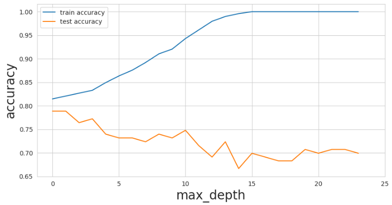 Train accuracy vs test accuracy
You'll notice that as max_depth values on the x-axis begin to increase, the training data accuracy starts improving a lot to a perfect score. In spite of this, the test data accuracy decreased from 0.78 to 0.70. This is a classic example of overfitting as the model becomes too complex.
Training and validation accuracy gap
The accuracy gap is a good way to know if overfitting has occurred in your program. This means that there is a wide gap between training data and validation data when it comes to accuracy.
As a guide, a 5% gap is what you should look for. Cases where you have more than this are often an indicator of overfitting: for example, our visualization above shows that when our max_depth value was at 2o, our training accuracy was at 100% while our test accuracy was 70%.
How to Prevent Overfitting
Collect more training data
As discussed above, insufficient training data can cause overfitting as the model cannot capture the relevant patterns and intricacies represented in the data.
Machine learning generally requires thousands or millions of records in your dataset for training. With this, there will be enough patterns to capture. You can identify outliers or noise more easily if you've done proper cleaning on the dataset using relevant techniques.
Use regularization techniques
Regularization techniques involve simplifying models by penalizing less influential features. These penalties are embedded in the model's loss function.
Regularization techniques for the decision tree model above include pruning, cost complexity pruning, and others.
Pruning is a technique that involves removing unnecessary branches from the decision tree. For example, we can set a minimum number of customers on a leaf, such as 20. This prevents the tree from making decisions based on a very small group of customers.
Cost complexity involves removing branches from the tree based on their complexity. This controls the trade-off between tree complexity and accuracy.
Ensembling
Ensembling entails combining several machine learning models to contribute their strengths and unique perspectives to make a prediction.
Ensembling leverages the wisdom of the crowd to make more accurate predictions on unseen data, which improves generalization and reduces the risk of overfitting.
Popular ensemble methods include bagging, boosting, and stacking, which have been successful in a wide range of machine-learning tasks.
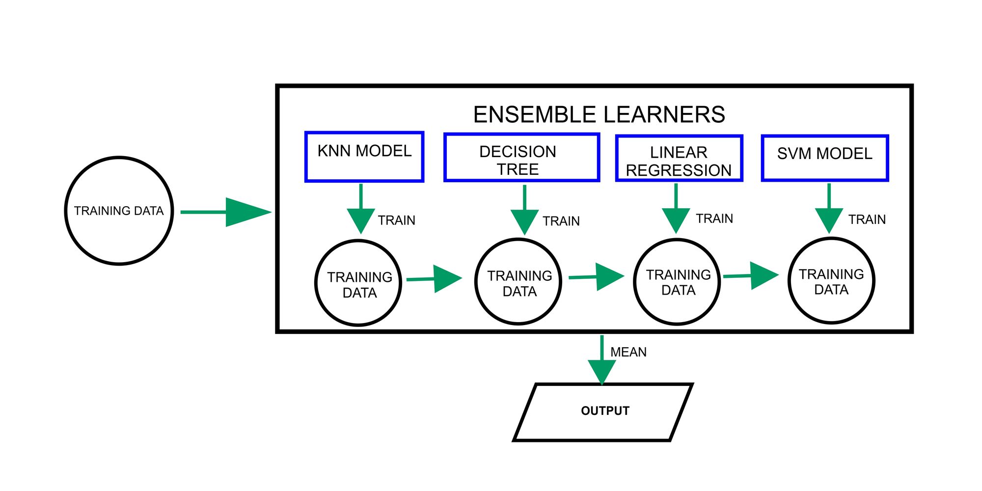 Diagram showing how ensembling works
The diagram above shows how the ensembling method combines various machine learning models for making predictions. Each model is trained independently on its respective subset of data. The predictions for individual models are then combined or the mean is gotten to make a final prediction.
Conclusion
Overfitting happens when a model fits training data too closely, resulting in great training performance but poor generalization. Overfitting can be problematic as it yields incorrect predictions.
This can be caused by a lack of training data, an overly complex model, or noisy data. Diagnosis involves assessing the training-validation accuracy gap, using visualizations to scrutinize model behavior, and so on.
Prevention strategies include collecting more training data, using regularization techniques, and employing ensemble methods. These approaches ensure models generalize well and make accurate predictions for informed decisions.
Thank you for reading! Please follow me on LinkedIn where I also post more data related content.
References:
- Siddhardhan. "Overfitting in Machine Learning | Causes for Overfitting and its Prevention" [Video]. Retrieved from https://www.youtube.com/watch?v=gy8kXdd6K-o
- Udacity. "Ensemble Learners" [Video]. Retrieved from https://www.youtube.com/watch?v=Un9zObFjBH0
- White Board Machine Learning. "Overfitting in Decision Trees" [Video]. Retrieved from https://www.youtube.com/watch?v=eU4X-dL8nYo