
By Peter Gleeson
Laplace, Bayes, and machine learning today
It may not be a question that you were worrying much about. After all, it appears to happen every day without fail.
But what is the probability the sun will rise tomorrow?
Believe it or not, this question was given consideration by one of mathematics’ all-time greats Pierre-Simon Laplace in his pioneering work of 1814, “Essai philosophique sur les probabilités”.
Fundamentally, Laplace’s treatment of the question was intended to illustrate a more general concept. It was not a serious attempt to estimate whether the sun will, in fact, rise.
In his essay, Laplace describes a framework for probabilistic reasoning that today we recognise as Bayesian.
The Bayesian approach forms a keystone in many modern machine learning algorithms. But the computational power required to make use of these methods has only been available since the latter half of the 20th Century.
(So far, it appears current state-of-the-art AI is keeping quiet on the issue of tomorrow’s sunrise.)
Laplace’s ideas are still relevant today, despite being developed more than two centuries ago. This article will review some of these ideas, and show how they are used in modern applications, perhaps envisaged by Laplace’s contemporaries.
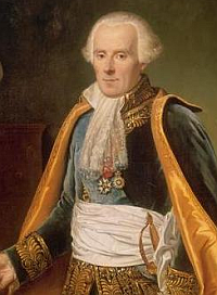
Pierre-Simon Laplace
Born in the small Normandy commune of Beaumont-en-Auge in 1749, Pierre-Simon Laplace was initially marked out to become a theologian.
However, while studying at the University of Caen, he discovered a brilliant aptitude for mathematics. He transferred to Paris, where he impressed the great mathematician and physicist Jean le Rond d’Alembert.
At the age of 24, Laplace was elected to the prestigious Académie des Sciences.
Laplace was an astonishingly prolific scientist and mathematician. Amongst his many contributions, his work on probability, planetary motion, and mathematical physics stand out. He counted figures such as Antoine Lavoisier, Jean d’Alembert, Siméon Poisson, and even Napoleon Bonaparte, as his collaborators, advisers, and students.
Laplace’s “Essai philosophique sur les probabilités” was based upon a lecture he delivered in 1795. It provided a general overview of ideas contained within his work “Théorie analytique des probabilités”, published two years earlier in 1812.
In “Essai philosophique”, Laplace provides ten principles of probability. The first few cover basic definitions, and how to calculate probabilities relating to independent and dependent events.
Principles eight, nine, and ten concern the application of probability to what we might describe today as cost-benefit analysis.
The sixth is an important generalization of Thomas Bayes’ eponymous theorem of 1763.
It states that, for a given event, the likelihood of each possible cause is found by multiplying the prior probability of that cause by a fraction.
This fraction is the probability of the event arising from that particular cause, divided by the probability of the event occurring by any cause.

This theorem’s influence within machine learning cannot be overstated.
The seventh principle is the one that has caused the most controversy since its publication. However, the actual wording is innocuous enough.
Rather, it is Laplace’s choice of discussing the probability of the sun rising the next day by way of illustrative example that has in turn drawn derision and objection over the following two centuries.
The rule of succession is still used today under various guises, and sometimes in the form Laplace originally described.
In fact, the rule of succession represents an important early step in applying Bayesian thinking to systems for which we have very limited data and little or no prior knowledge. This is a starting point often faced in modern machine learning problems.
Laplace’s rule of succession
The seventh principle of probability given in Laplace’s “Essai philosophique” is, in essence, straightforward.
It states that the probability of a given event occurring is found by summing the probability of each of its potential causes multiplied by the probability of that cause giving rise to the event in question.
Laplace then proceeds to outline an example based upon drawing balls from urns. So far, so good. Nothing contentious yet.
However, he then describes how to proceed with estimating the probability of an event occurring in situations where we have limited (or indeed no) prior knowledge about what that probability might be.
“On trouve ainsi qu’un événement étant arrivé de suite un nombre quelconque de fois , la probabilité qu’il arrivera encore la fois suivante est égale à ce nombre augmenté de l’unité, divisé par le même nombre augmenté de deux unités.”
Which translates in English: “So, one finds for a event which has occurred any number of times until now, the probability it will occur again the next time is equal to this number increased by one, divided by the same number increased by two”.
Or, in math notation:

That is, given s successes out of n trials, the probability of success on the next trial is approximately (s+1)/(n+2).
To make his point, Laplace doesn’t hold back:
“… par exemple, remonter la plus ancienne époque de l’histoire à cinq mille ans, ou à 1,826,213 jours, et le soleil s’étant levé constamment dans cet intervalle, à chaque révolution de vingtquatre heures, il y a 1,826,214 à parier contre un qu’il se lèvera encore demain”
Which translates as: “…for example, given the sun has risen every day for the last 5000 years — or 1,826,213 days — the probability it will rise tomorrow is 1,826,214 / 1,826,215”.
At 99.9%, that’s a pretty certain bet. And it only becomes more certain each day the sun continues to rise.
Yet Laplace acknowledges that, for someone who understands the mechanism by which the sun rises and sees no reason why it should cease to function, even this probability is unreasonably low.
And it turns out that this qualification is perhaps just as important as the actual rule itself. After all, it hints at the fact that our prior knowledge of a system is encoded in the assumptions we make when assigning probabilities to each of its potential outcomes.
This is true in machine learning today, especially when we try learning from limited or incomplete training data.
But what is the rationale behind Laplace’s rule of succession, and how does it live on in some of today’s most popular machine learning algorithms?
Nothing is impossible?
To better understand the significance of Laplace’s rule, we need to consider what it means to have very little prior knowledge about a system.
Say you have one of Laplace’s urns, which you know to contain at least one red ball. You know nothing else about the contents of the urn “system”. Perhaps it contains many different colors, perhaps it only contains that one red ball.
Draw one ball from the urn. You know the probability that it will be red is greater than zero, and either less than or equal to one.
But, as you don’t know whether the urn contains other colors, you cannot say the probability of drawing red certainly equals one. You simply cannot rule out any other possibility.
So, how do you estimate the probability of drawing a red ball from the urn?
Well, according to Laplace’s rule of succession, you can model drawing a ball from the urn as a Bernoulli trial with two possible outcomes: “red” and “not-red”.
Before we’ve drawn anything from the urn, we’ve already allowed for two potential outcomes to exist. In so doing, we’ve effectively “pseudo-counted” two imaginary draws from the urn, observing each outcome once.
This gives each outcome (“red” and “not-red”) a probability of 1/2.
As the number of draws from the urn increases, the effect of these pseudo-counts becomes less and less important. If the first ball drawn is red, you update the probability of the next one being red to (1+1)/(1+2) = 2/3.
If the next ball is red, the probability updates to 3/4. If you keep drawing red, the probability reaches ever closer to 1.
In today’s language, probability concerns a sample space. This is a mathematical set of all possible outcomes for a given “experiment” (a process that selects one of the outcomes).
Probability was put on a formal axiomatic basis by Andrey Kolmogorov in the 1930s. Kolmogorov’s axioms make it easy to prove that a sample space must contain at least one element.
Kolmogorov also defines probability as a measure that returns a real valued number between zero and one for all elements of the sample space.
Naturally, probability makes a useful way to model real world systems, especially when you assume complete knowledge about the contents of the sample space.
But when we don’t understand the system at hand, we don’t know the sample space — apart from that it must contain at least one element. This is a common starting point in many machine learning contexts. We have to learn the contents of the sample space as we go.
Therefore, we ought to allow the sample space to contain at least one extra, catch-all element — or, if you like, the “unknown unknown”. Laplace’s rule of succession tells us to assign the “unknown unknown” a probability of 1/n_+_2, after n repeated observations of known events.
Although in many cases it is convenient to ignore the possibility of unknown unknowns, there are epistemological grounds for always allowing such eventualities to exist.
One such argument is known as Cromwell’s Rule, coined by the late Dennis Lindley. Quoting the 17th century’s Oliver Cromwell:
“I beseech you, in the bowels of Christ, think it possible that you may be mistaken”
This rather dramatic statement asks us to allow a remote possibility for the unexpected to occur. In the language of Bayesian probability, this amounts to requiring us to always consider a non-zero prior.
Because if your prior probability is set to zero, no amount of evidence will ever convince you otherwise. After all, even the strongest evidence to the contrary will still yield a posterior probability of zero, when multiplied by zero.
Objections, and a defence of Laplace
It may come as little surprise to learn that Laplace’s sunrise example attracted much criticism from his contemporaries.
People objected to the perceived simplicity — naivety, even — of Laplace’s assumptions. The idea that there was a 1/1,826,215 probability the sun would not rise the following day seemed absurd.
It is tempting to believe that, given a large number of trials, a non-zero probability event must happen. And therefore, observing so many consecutive sunrises without a single failure surely implies Laplace’s estimate is an overestimate?
For example, you might expect that after a million trials, you’d have observed a one-in-a-million event — almost guaranteed by definition! What’s the probability of doing otherwise?
Well, you wouldn’t be astonished if you tossed a fair coin twice without landing heads. Nor would it be cause for concern if you rolled a die six times, and never saw the number six. These are events with probability 1/2 and 1/6 respectively, but that absolutely does not guarantee their occurrence in the first two and six trials.
A result attributed to Bernoulli back in the 17th Century finds the limit as the probability 1/n and number of trials n grow very large:

Although on average you will have observed at least one occurrence of an event with probability 1/n after n trials, there is still a greater than 1/3 chance you will not.
Likewise, if the true probability of the sun failing to rise were indeed 1/1,826,215, then we perhaps shouldn’t be so surprised such an occurrence has never been recorded in history.
And, arguably, Laplace’s qualification is too generous.
It is true that, for a person who claims to understand the mechanism by which the sun rises every day, the probability of it failing to do so must be much closer to zero.
Yet to assume an understanding of such a mechanism requires us to possess prior knowledge of the system, beyond that which we have observed. This is because such a mechanism is implicitly assumed constant — in other words, true for all time.
This assumption lets us, in a sense, “conjure up” an unlimited number of observations — on top of those we have actually observed. It’s an assumption called for by none other than Isaac Newton, at the beginning of the third book in his famous “Philosophiae Naturalis Principia Mathematica”.
Newton outlines four “Rules of Reasoning in Philosophy”. The fourth rule claims we can regard propositions derived from previous observations as “very nearly true”, until contradicted by future observations.
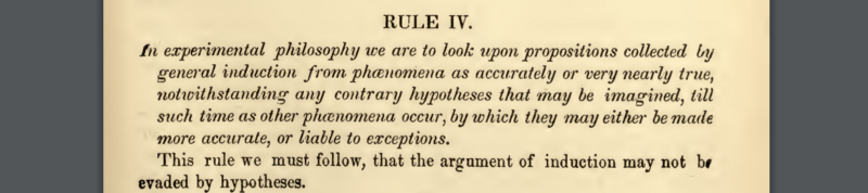
Such an assumption was crucial for the scientific revolution, despite being a kick in the teeth for philosophers such as David Hume, who famously argued for the problem of induction.
It is this epistemological compromise that lets us do useful science and, in turn, invent technology. Somewhere along the line, as we see the estimated probability of the sun failing to rise diminish ever closer to zero, we allow ourselves to “round down” and claim a fully fledged scientific truth.
But all of this presumably lies beyond the scope of the point Laplace originally sought to make.
Indeed, his choice of a sunrise example is unfortunate. The rule of succession really comes into its own when applied to completely unknown “black-box” systems for which we have zero (or very few) observations.
This is because the rule of succession offers an early example of a non-informative prior.
How to assume as little as possible
Bayesian probability is a keystone concept in modern machine learning. Algorithms such as Naive Bayes classification, Expectation Maximisation, Variational Inference and Markov Chain Monte Carlo are amongst the most popular in use today.
Bayesian probability generally refers to an interpretation of probability where you update your (often subjective) belief in the light of new evidence.
Two key concepts are prior and posterior probabilities.
Posterior probabilities are those we ascribe to after updating our beliefs in the face of new evidence.
Prior probabilities (or ‘priors’) are those we hold to be true before seeing new evidence.
Data scientists are interested in how we assign prior probabilities to events in the absence of any previous knowledge at all. This is a typical starting point for many problems in machine learning and predictive analytics.
Priors can be informative, in the sense they come with “opinions” about the probability of different events. These “opinions” can be strong or weak, and are usually based on past observations or otherwise reasonable assumptions. These are invaluable in situations where we want to train our machine learning model quickly.
However, priors can also be non-informative. This means they assume as little as possible about the respective probabilities of an event. These are useful in situations where we want our machine learning model to learn from a blank state.
So we must ask: how do you measure how “informative” a prior probability distribution is?
Information theory provides an answer. This is a branch of mathematics that concerns how information is measured and communicated.
Information can be thought of in terms of certainty, or a lack thereof.
After all, in an everyday sense, the more information you have about some event, the more certain you are about its outcome. Less information equates to less certainty. This means that information theory and probability theory are inextricably linked.
Information entropy is a fundamental concept in information theory. It serves as a measure of the uncertainty inherent to a given probability distribution. A probability distribution with high entropy is one for which the outcome is more uncertain.

Perhaps intuitively, you can reason that a uniform probability distribution — a distribution for which each event is equally likely — has the highest possible entropy. For example, if you flipped a fair coin and a biased coin, which outcome would you be least certain about?
Information entropy provides a formal means of quantifying this, and if you know some calculus, you can check out the proof here.
So the uniform distribution is, in a very real sense, the least informative distribution possible. And for that reason, it makes an obvious choice for an uninformative prior.
Perhaps you’ve spotted how Laplace’s rule of succession effectively amounts to using a uniform prior? By adding one success and one failure before we’ve even observed any outcomes, we’re using a uniform probability distribution to represent our “prior” belief about the system.
Then, as we observe more and more outcomes, the weight of the evidence increasingly overpowers the prior.
Case study: Naive Bayes classification
Today, Laplace’s rule of succession is generalised to additive smoothing and pseudo-counting.
These are techniques which allow us to use non-zero probabilities for events not observed in training data. This is an essential part of how machine learning algorithms are able to generalize when faced with inputs not seen previously.
For instance, take Naive Bayes classification.
This is a simple yet effective algorithm that can classify textual and other suitably tokenized data, using Bayes’ theorem.
The algorithm is trained on a corpus of pre-classified data, in which each document consists of a set of words or “features”. The algorithm begins by estimating the probability of each feature, given a certain class.
Using Bayes’ theorem (and some very naive assumptions about feature independence), the algorithm can then approximate the relative probabilities of each class, given the features observed in a previously unseen document.

An important step in Naive Bayes classification is estimating the probability of a feature being observed within a given class. This can be done by calculating the frequency at which the feature is observed in each of that class’s records in the training data.
For instance, the word “Python” might appear in 12% of all documents classed as “programming”, compared to 1% of all documents classed as “start-up”. The word “learn” might appear in 10% of programming documents and 20% of all start-up documents.
Take the sentence “learn Python”.
Using these frequencies, we find the probability of the sentence being classed as “programming” equals 0.12 ×0.10 = 0.012, and the probability of it being classed as “start-up” is 0.01×0.20 = 0.002.
Therefore, “programming” is the more likely of these two classes.
But this frequency-based approach runs into trouble whenever we consider a feature which never occurs in a given class. This would mean it has a frequency of zero.
Naive Bayes classification requires us to multiply probabilities, but multiplying anything by zero will, of course, always yield zero.
So, what happens if a previously unseen document does contain a word never observed in a given class in the training data? That class will be deemed impossible — no matter how frequently every other word in the document occurs in that class.
Additive smoothing
An approach called additive smoothing offers a solution. Instead of allowing for zero frequencies, we add a small constant to the numerator. This prevents unseen class/feature combinations from derailing the classifier.
When this constant equals one, additive smoothing is the same as applying Laplace’s rule of succession.
As well as Naive Bayes classification, additive smoothing is used in other probabilistic machine learning contexts. Examples include problems in language modelling, neural networks, and hidden Markov models.
In mathematical terms, additive smoothing amounts to using a beta distribution as a conjugate prior for carrying out Bayesian inference with binomial and geometric distributions.
The beta distribution is a family of probability distributions defined over the interval [0,1]. It takes two shape parameters, α and β. Laplace’s rule of succession corresponds to setting α = 1 and β = 1.
As discussed above, the beta(1,1) distribution is the one for which information entropy is maximised. However, there are alternative priors for cases in which the assumption of one success and one failure are not valid.
For instance, Haldane’s prior is defined as a beta(0,0) distribution. It applies in cases when we are not even sure if we can allow for a binary outcome. Haldane’s prior places an infinite amount of “weight” on zero and one.
Jeffrey’s prior, the beta(0.5, 0.5) distribution, is another non-informative prior. It has the helpful property that it remains invariant under reparameterization. Its derivation is beyond the scope of this article, but if you are interested, check out this thread.
The legacy of ideas
Personally, I find it fascinating how some of the earliest ideas in probability and statistics have survived years of contention, and still find widespread use in modern machine learning.
It is extraordinary to realise that the influence of ideas developed more than two centuries ago is still being felt today. Machine learning and data science have gained real mainstream momentum in the last decade or so. But the foundations upon which they are built were laid long before the first computers were even close to realization.
It’s no coincidence that such ideas border on the philosophy of knowledge. This becomes especially relevant as machines become more and more intelligent. At what point might the focus shift onto our philosophy of consciousness?
Finally, what would Laplace and his contemporaries make of machine learning today? It’s tempting to suggest they’d be astounded by the progress that’s been made.
But that would probably be a disservice to their foresight. After all, the French philosopher René Descartes had written of a mechanistic philosophy back in the 17th Century. Describing a hypothetical machine:
“Je désire que vous considériez … toutes les fonctions que j’ai attribuées à cette machine, comme … la réception de la lumière, des sons, des odeurs, des goûts … l’empreinte de ces idées dans la mémoire … et enfin les mouvements extérieurs … qu’ils imitent le plus parfaitement possible ceux d’un vrai homme … considériez que ces fonctions … de la seule disposition de ses organes, ni plus ni moins que font les mouvements d’une horloge … de celle de ses contrepoids et de ses roues”
Which translates as: “I desire that you consider that all the functions I’ve attributed to this machine such as… the reception of light, sound, smell and taste… the imprint of these ideas in the memory… and finally the external movements which imitate as perfectly as possible those of a true human…Consider that these functions are only under the control of the organs, no more or less than the movements of a clock are to its counterweights and wheels”
The passage above describes a hypothetical machine capable of responding to stimuli and behaving like a “true human”. It was published in Descartes’ 1664 work “Traité de l’homme” — a full 150 years before Laplace’s “Essai philosophique sur les probabilités”.
Indeed, the 18th and early 19th Centuries saw the construction of incredibly sophisticated automata by inventors such as Pierre Jaquet-Droz and Henri Maillardet. These clockwork androids could be “programmed” to write, draw, and play music.
So there is no doubting that Laplace and his contemporaries could conceive of the notion of an intelligent machine. And it surely would not have escaped their notice how progress made in the field of probability might be applied to machine intelligence.
Right at the beginning of “Essai philosophique”, Laplace writes of a hypothetical super-intelligence, retrospectively named “Laplace’s Demon”:
“Une intelligence qui, pour un instant donné, connaîtrait toutes les forces dont la nature est animée, et la situation respective des êtres qui la composent, si d’ailleurs elle était assez vaste pour sou- mettre ces données à l’analyse … rien ne serait incertain pour elle, et l’avenir comme le passé, serait présent à ses yeux”
Which translates as: “An intelligence, which in a given moment, knows all the forces by which nature is animated, and the respective situation of the beings which compose it, and if it were large enough to submit these data to analysis … nothing would be uncertain to it, and the future as the past, would be present in its eyes”.
Could Laplace’s Demon be realized as one of Descartes’ intelligent machines? Modern sensibilities overwhelmingly suggest no.
Yet Laplace’s premise envisaged on a smaller scale may soon become a reality, thanks in no small part to his own pioneering work in the field of probability.
Meanwhile, the sun will (probably) continue to rise.