By Samuel A. Olubiyo
Microsoft Excel is a very powerful tool that you can use to analyze and visualize data.
In this tutorial, you will learn how to build a simple Excel Dashboard that visualizes important data from a large dataset.
The dataset we'll be working with is the transaction records of a super store for a period of four years. Our goal is to gain important insights from the dataset and visualize those insights graphically with Microsoft Excel.
This tutorial is tailored for those who are already familiar with Excel. In it, you will learn:
- How to format dates in Excel using the TEXT function.
- How to sort the entire data set.
- How to create multiple Pivot Tables on the same worksheet
- How to create charts based on the Pivot Table.
- How to create slicers to filter data, and finally,
- How to use conditional formatting.
In order to make the most of this tutorial, I have provided a data set for you to use. You can download it here.
If you're new to data analysis and visualization with Excel, the freeCodeCamp website contains a lot of tutorials for beginners. Here is a link to some articles on Excel from beginner to advanced if you need to brush up on your skills.
Our Dataset
After downloading the Excel file and opening it, you will notice one thing instantly: The data is huge! It is a data set containing the transactions of a superstore for a period of four years (from 2014 to 2017).
This Excel file is made up of 9995 rows and 21 columns. We can’t gain any useful insights from this data set just by staring at it, which is why we need to analyze and visualize it.
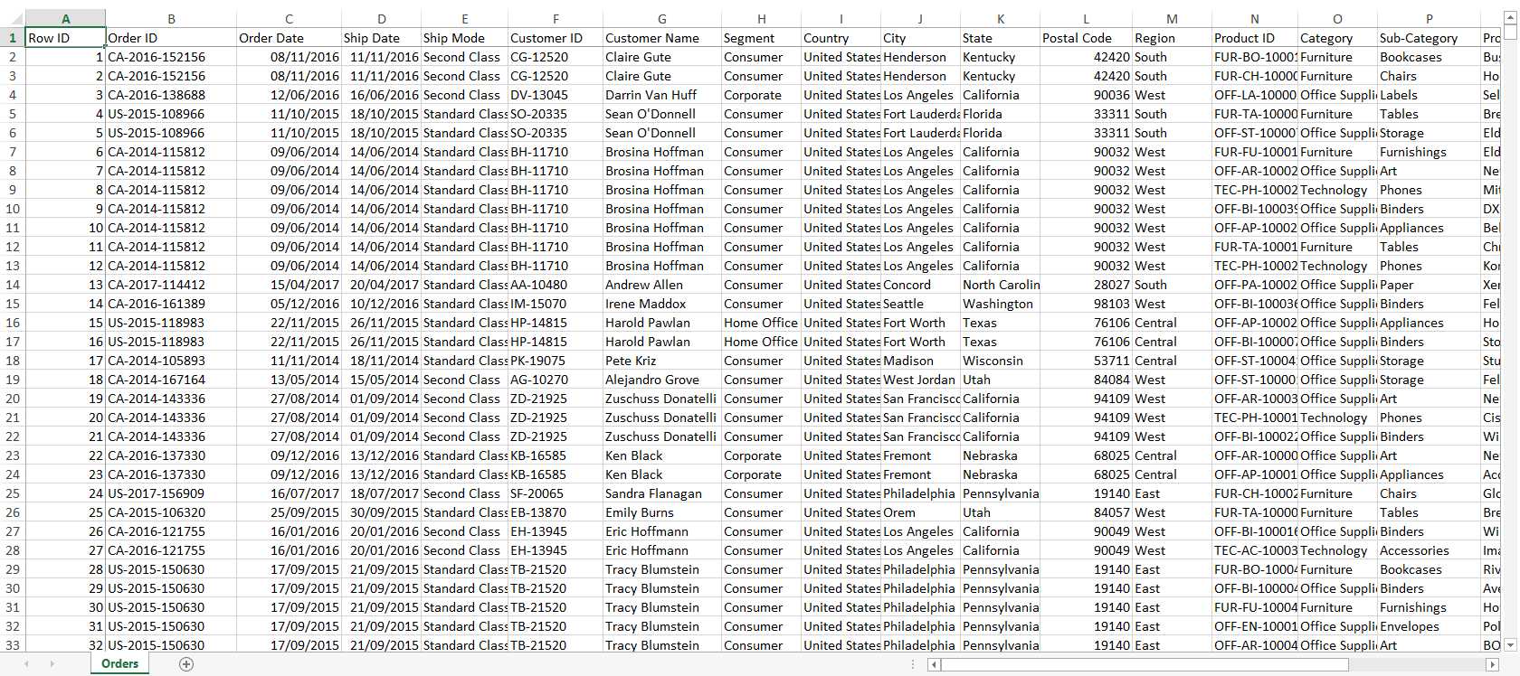 Screenshot of the dataset
The easiest way to do this is by using Pivot Tables. A Pivot Table is one of Microsoft Excel's powerful tools you can use to calculate, analyze and summarize data. It helps you see comparisons, trends, and patterns in your data and you will learn how to use it in this tutorial.
Before we continue, let's take a look at the data set again: column C contains the order dates for each product sold. The order date column is important in this tutorial, because we need to sort the entire dataset based on the dates each customer ordered a product.
How to Format Dates in Excel Using the TEXT Function.
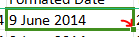
In our dataset, the dates are arranged haphazardly and the date formatting makes it hard to tell exactly when each customer ordered a product. To fix this, we'll use the TEXT function to convert the dates to text.
Before you do this, insert a new column beside column C. This will be your new column D and where the newly formatted dates will reside. You can give it a new name – in my own case, I named it “Formatted Dates.”
After that is done, insert the formula in the screenshot below and press enter:
 Formula to convert dates into text
Or just copy and paste the formula below:
=TEXT(C2, "d mmmm yyyy")
Of course, the formula only works for the first cell in the column. To repeat it across the entire column, just double-tap the little node at the right end of the cell when it's highlighted (as you can see in the below screenshot):
 Tap on the node to fill the remaining cells in the column automatically
Now, you should have dates in a more readable format across column D.
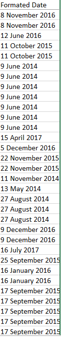 The dates in a more readable format
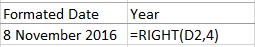
For the purpose of this analysis, we need to extract the years from the dates we have just formatted. To do this, create a new column beside column D, this will be your new column E. Name the column as you like, but in my case, I named it “Year”.
Now use the formula in the screenshot below and press enter:
 Formula to get the year from the date
Or simply copy and paste the formula below:
=RIGHT(D2,4)
This will extract the year at the end of the date. Double-tap the node at the end of the cell to repeat it across the entire column. You should get a similar result as shown in the screenshot below:
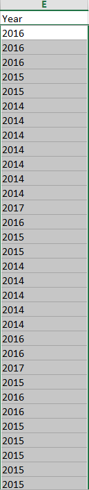 Screenshot showing the extracted year
How to Sort the Entire Dataset
The next step in this tutorial is to sort the entire data set based on the newly extracted Year column.
Highlight the entire Year column and go to the sort tab, as you can see in the screenshot below:
 Sorting the dataset
Leave all options at default and press OK.
Now the entire data set should be sorted.
How to Create Multiple Pivot Tables on the Same Worksheet
The next step in this tutorial is to create the pivot tables we'll use to make sense of this data.
Go to the insert tab and click on Pivot Table. A dialogue box should pop up asking you for the range of the data you want the pivot table to be created from – which by default is the entire data set.
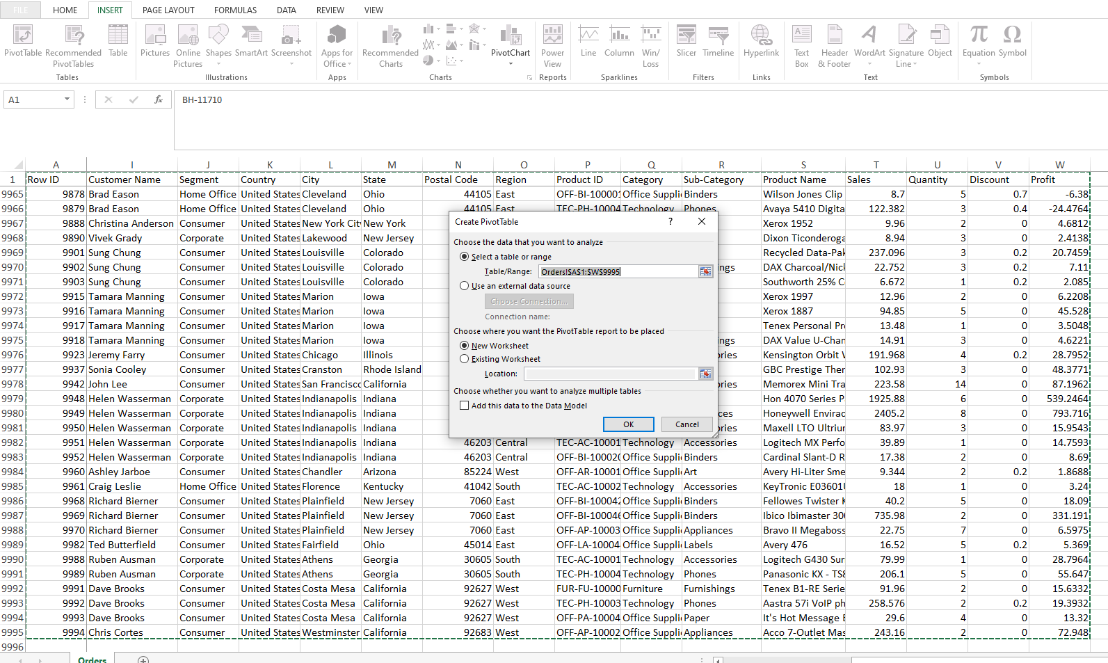 Creating a Pivot Table
You will also have options to use the existing worksheet to create the pivot table or a new worksheet. Select the new worksheet option and press OK.
You should have a result like you can see in the screenshot below:
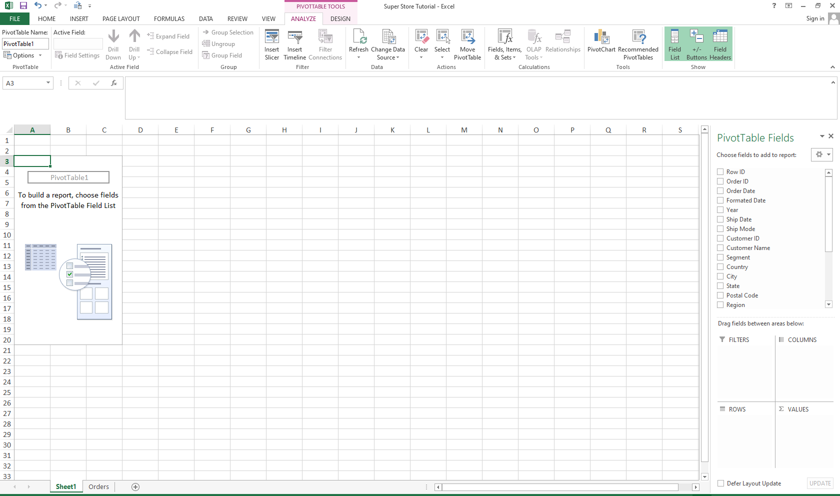 The Pivot Table Worksheet
From here things start to get interesting.
For this exercise, I am only interested in three things:
- The category of products with the highest sales for each of the four years (2014 to 2017)
- Which sub-category has the highest sales
- Which region drives the most sales to this super store.
I also want to visualize this information using graphs and charts. Thankfully, Excel has the tools we need to achieve all these.
In case you don’t know how to create a Pivot Table, here is a comprehensive freeCodeCamp article teaching you how to do that.
So we need to create three Pivot Tables, one for the sales by category, one for the sales by sub-category, and one for the sales by region.
To create the first table, simply select sales and category from the PivotTable Fields at the right hand side of your screen.
After creating the first Pivot Table, to add another table on the same worksheet, simply go to the insert tab and click on Pivot Table, then go to the original worksheet with the dataset and highlight everything, click OK.
Repeat the step to create the last table for the sales by region.
You should have three tables as shown in the screenshot below:
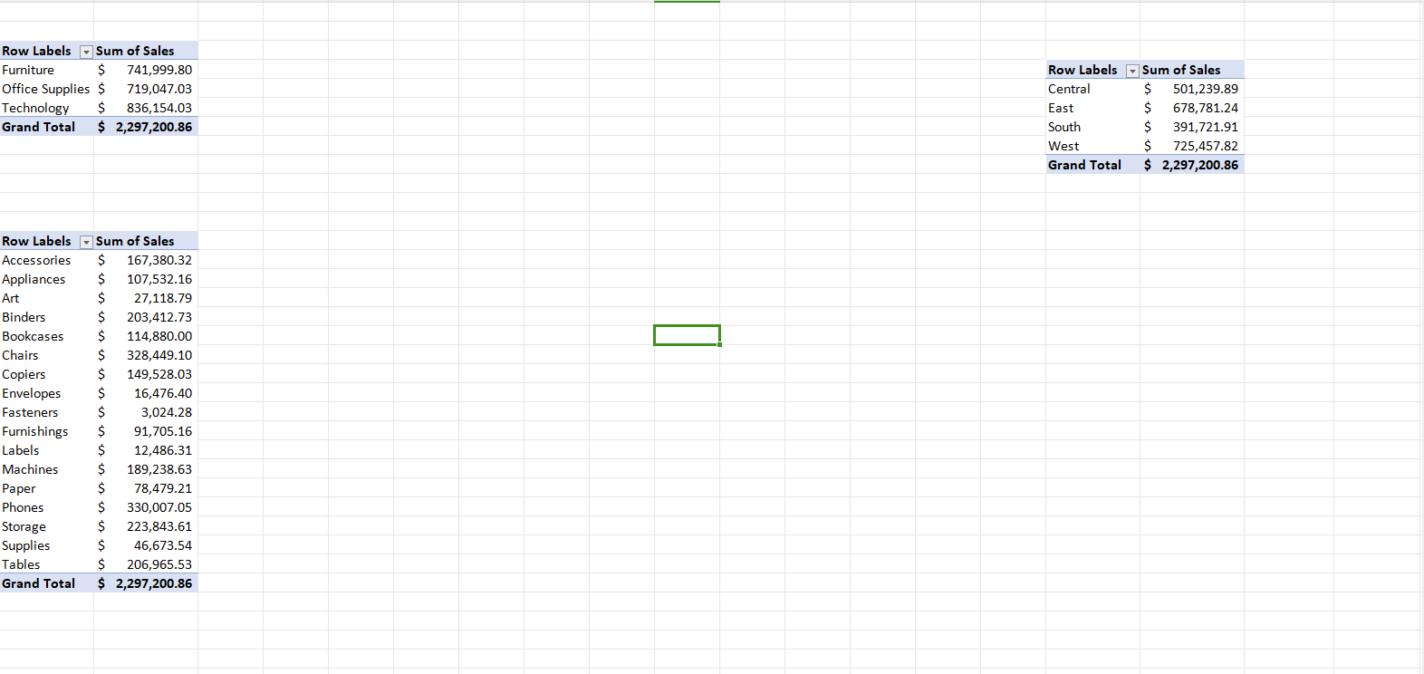 Screenshot showing all three Pivot Tables
How to Create Charts Based on the Pivot Table
The next step is to create the charts to visualize what is represented in the Pivot Tables. This is quite straightforward – just highlight each table and click the insert tab to insert the chart of your choice.
I used a pie chart for the sales by category table, and column charts for the other two tables on the worksheet. But you can use whatever chart(s) you want.
If you follow my steps exactly, you should have a result similar to the screenshot below:
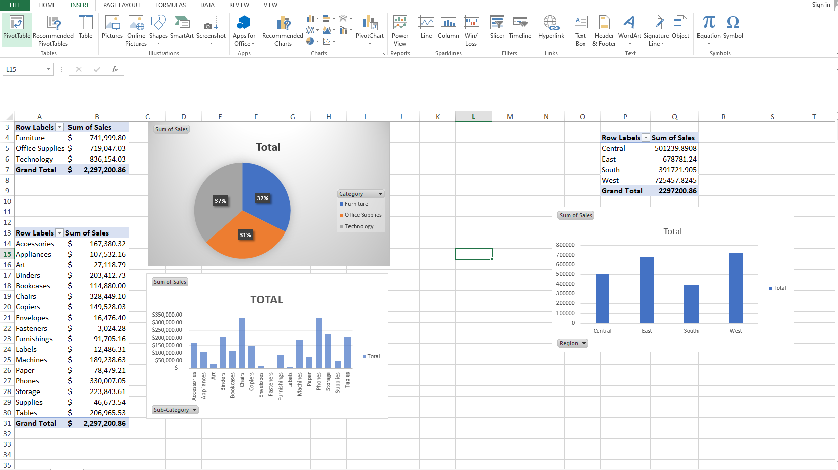 Screenshot showing all the charts
How to Create Slicers to Filter Data
The next step is to use slicers to filter each table by the year so that we can see what the total sales for each category, sub-category, and region are by year.
To do this, highlight each table and click on the analyze tab, then click on the slicer button as shown in this screenshot:
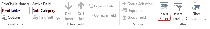 Creating a slicer
You'll see a list of options. Look for Year, and click it.
Now you should have a slicer for the years 2014 to 2017. Clicking on the corresponding button for each year will filter the table and show the sales for the year. Here is what it should look like:
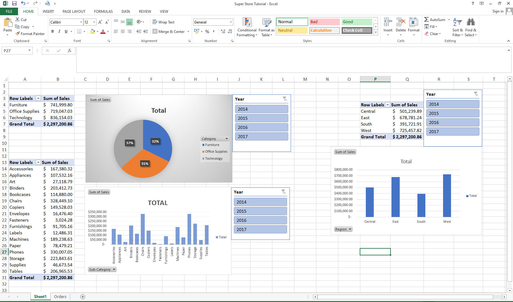 Screenshot showing all the slicers
How to Use Conditional Formatting
Finally, you can use conditional formatting to indicate the highest and lowest values on each table. You can play around with this as you like.
To use conditional formatting, click on the conditional formatting tab, and use this screenshot as a guide:
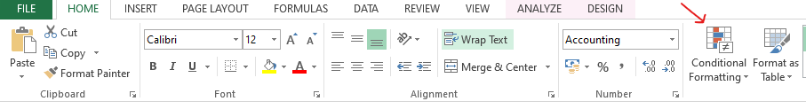 Using conditional formatting
Highlight the values you would like to use conditional formatting for. I used the color scales option to indicate the highest and lowest values by different colors, then I used the data bars option for the sales by sub-category table.
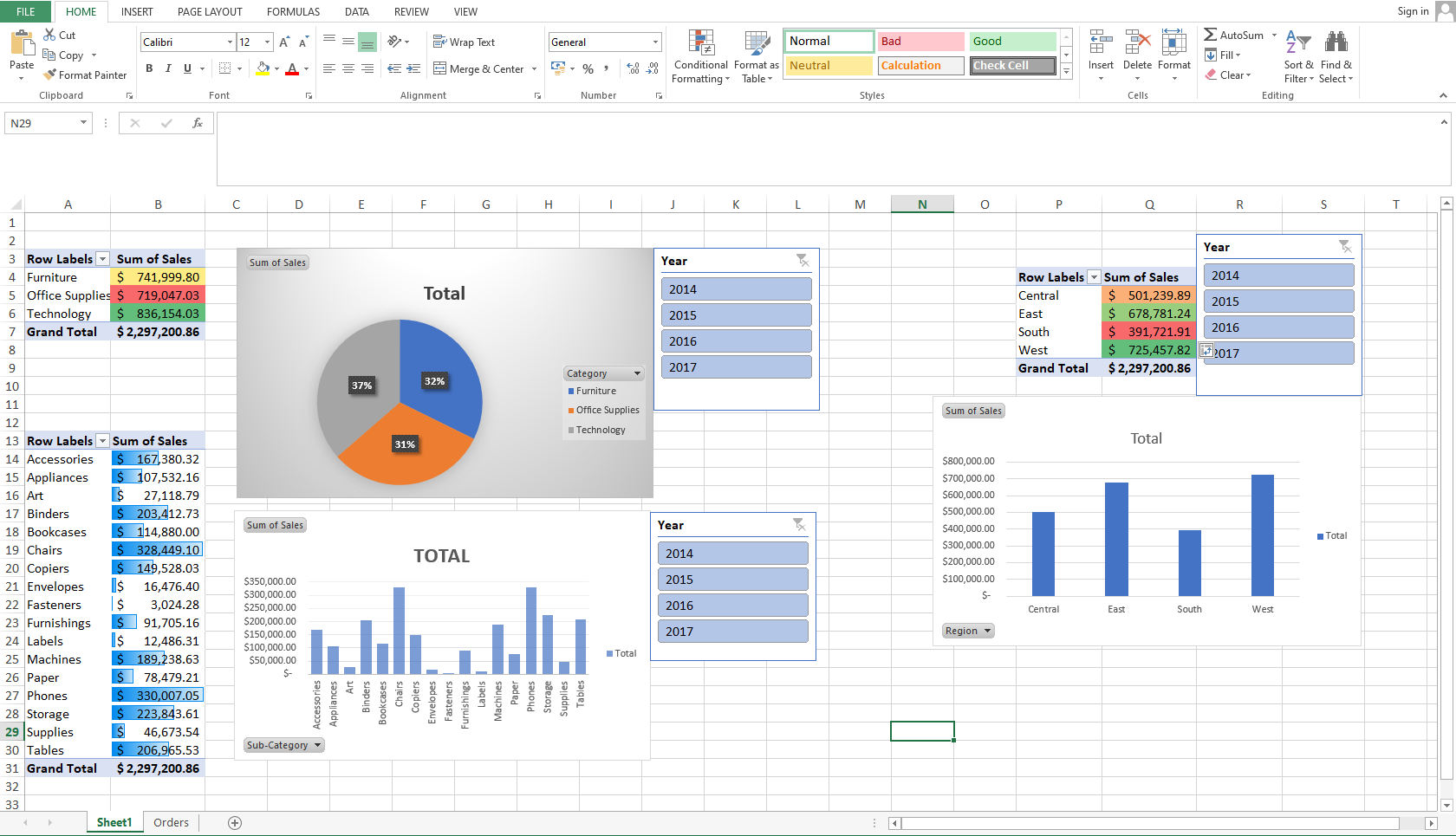
If you did exactly what I did, you should have something close to the screenshot below:
 The completed dashboard
Wrapping Up
This little project we have built together can be expanded to get more insights into the data set, this can prove very useful when making business decisions.
This dashboard we have built has revealed that the best selling category is electronics and the best selling sub-category is phones. I also learned that the most sales came from the western region just by glancing at this dashboard.
I hope this tutorial has been helpful. Here is the link to the completed version of this project – you can compare it with what you have built and see how well you did.
If you have any questions, you can reach out to me on X and LinkedIn. Thanks for reading.