
By Gregory V. Chapman
When dealing with Excel workbooks, data may be structured in a way that doesn’t fit your needs and objectives.
Sometimes, you may need to split the content of one cell into different cells. You may also need to do the opposite, combining data from multiple columns into one.
The second process is called concatenation. Most often, you use concatenation in Excel to join such data as names and addresses, display time, and date.
In this guide, we will look at concatenation in detail and examine the techniques that you can use in different situations.
What Does “Concatenate” Mean?
Generally, Excel enables you to combine data in two ways: you can either merge cells or concatenate their values.
The first option means turning multiple cells into one. As a result, you get a single large cell that is displayed across multiple columns or rows.
If you choose to concatenate cells instead, you won’t merge the cells themselves but combine their content.
Concatenation doesn’t impact cells but joins multiple values. For example, you can use this method to combine pieces of textual content from different cells. In Excel, such content is called text strings. You can also insert a number obtained from a formula in-between textual content.
For example, you may have your customers’ first names in column B, and their last names in column C. You may want column D to contain both their first and last names, but retyping their names manually is too time-consuming and inefficient.
In this case, you can use concatenation functions, like “CONCATENATE,” “CONCAT,” and “&.” Let’s consider each one of these formulas and figure out the differences.
How to Join Text Strings in Excel
CONCATENATE
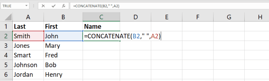
Excel lets you to join text strings in different ways. First of all, you can use the CONCATENATE function. In this case, your formula will look like this:
=CONCATENATE(X1,X2,X3)
X1, X2, and X3 are the cells that you want to join.
If you want to separate values of cells with spaces, you can add them in quotation marks, separated with commas:
=CONCATENATE(X1,“ ”,X2)
CONCAT
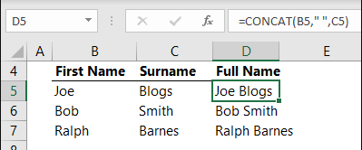
CONCATENATE is the oldest function of this kind and the only function you can use to join text strings when dealing with Excel 2013.
However, if you’re using a newer version of Excel, you might consider updated functions. The CONCATENATE function may also be unavailable in future versions. The CONCAT function works with Excel 2016 and Excel Mobile.
You can use this formula in the same way as CONCATENATE, but CONCAT is certainly easier to use because it’s shorter.
Here’s what the example above would look like with the CONCAT function:
=CONCAT(X1,X2,X3)
The “&” Operator

However, you may also choose not to use either of the formulas above and choose an even simpler option — the ampersand operator (&). This method of joining cells is recommended by Microsoft, and it’s much easier to use than the CONCAT and CONCATENATE functions.
Here’s an example of a formula that you can use:
=X1&X2&X3
If you want to separate the values of cells with spaces or commas, here’s what your formulae will look like:
=X1&“ ”&X2
=X1&“,”&X2
Using the “&” operator is a more convenient option. Besides, the “&” operator has no limitations regarding the number of strings that you can join.
In contrast, the CONCATENATE function is limited to 8,192 characters, which means that you can only use it to join up to 255 strings. However, sometimes you may want to use the CONCAT function to keep your formulae clean and to make them easier to read.
TEXTJOIN
Another function that you can use when combining textual content is TEXTJOIN. This function only works with the latest versions of Microsoft Office, and it offers some nice features.
First, you can choose how you want to separate the values of different cells, with no need to type these spaces, commas, or other symbols in the formula.
Secondly, the TEXTJOIN function enables you to ignore empty cells while including an array of arguments.
Here’s what the TEXTJOIN function looks like in Excel:
=TEXTJOIN(delimiter,ignore_empty,text1,[text2],...)
“Delimiter” is the separator that you want to use between different text strings, and “ignore_empty” can only take two values: TRUE or FALSE.
When using TEXTJOIN, you can still add cells manually, but in this case, the “&” operator would be a better choice. TEXTJOIN enables you to add a whole range of cells.
For example, here’s what function you can use to join text strings from the range A1:A4, separated with commas, ignoring empty values:
=TEXTJOIN(“,”,TRUE,A1:A4)
If you want to separate text strings with spaces and include empty values, the formula will look like this:
=TEXTJOIN(“ ”,FALSE,A1:A4)
How to Concatenate Text Strings With Line Breaks
Most often, Excel users need to separate text strings with spaces and punctuation marks. In this case, you can use formulae from the previous sections, depending on the chosen functions or operators.
However, sometimes you may need to separate text strings with a carriage return, or line break. For example, you may need to merge data and mailing addresses from separate columns or rows.
Unfortunately, you cannot put line breaks in formulae as easily as you do with punctuation marks because they are not regular characters. The good news is that you can include virtually any characters you want by using ASCII codes.
In this case, you should use the CHAR function. To include a line break on Windows, you should use CHAR(10), because 10 is the ASCII code for a line feed. On Mac, you should use CHAR(13), since 13 is the ASCII code for carriage return.
Keep in mind that you should also enable the “Wrap text” option to display the result correctly. Press Ctrl+1, then choose the “Alignment” tab in the “Format Cells” menu and then check the “Wrap text” box.
How to Concatenate Columns
To concatenate multiple columns, you can write a regular concatenation formula in the first cell, and then drag the fill handle to copy it to other cells.
To do it quickly, you can select the cell that contains the necessary formula, and then double-click the fill handle. Excel decides how far cells should be copied after your double click based on which cells are present in your formula. Therefore, if your table contains empty cells, you may need to drag the fill handle manually.
How to Concatenate a Range of Cells
Given that the CONCATENATE and CONCAT functions only accept single-cell references in arguments, joining values from multiple cells can be a challenge.
To quickly select multiple cells, you can press Ctrl and then click on each of the cells that you want to combine.
However, if you’re dealing with too many cells, this method may also be too time-consuming. In this case, you can use the TRANSPOSE function, which looks like this:
=TRANSPOSE(X1:Xn)
Type the TRANSPOSE formula in a cell where you want to include the concatenated range, then click on the formula bar, and press F9 to replace your formula with concatenated values. After this, you should delete the curly braces around the array values, type =CONCAT( before the first value, and add a closing parenthesis after the last value.
Things to Keep in Mind about Concatenating
Don’t forget to put commas between the concatenated items. For example, if you want to get the phrase “write my research paper,” your formula should be =CONCAT(“write”,“ ”,”my”,“ ”,”research”,“ ”,“paper”).
In this example, all items are also separated with designated spaces. You can also include extra spaces after each text string to avoid typing them separately in formulae.
If you type =CONCAT(“Hi”“there”), without a comma, the result will look like this: Hi”there. An extra quotation mark will appear because there’s no comma between the arguments.
If you see the “#NAME?” error instead of the desired result, it likely means that you forgot to include some quotation marks. The “#VALUE!” error means that some of the arguments are invalid.
You should also keep in mind that concatenate functions always return a text string, even if some cells contain numerical values. You can also convert numbers to text by using the TEXT function and use different formulae to set the format of numbers that you want to combine with text or symbols.
For example, if your A2 cell contains the number 13.6 and you want to display it as a dollar amount, your formula should be =TEXT(A2,“$0.00”). As a result, you will get $13.60.
Wrapping Up
Excel lets you to join text strings by using different functions, such as CONCATENATE, CONCAT, and the “&” operator.
While you can only use the CONCATENATE function in Excel 2013, the newer versions of Excel support a simple “&” operator that is much easier to use.
When concatenating values of different cells, pay attention to quotation marks and commas because they are very important for displaying the results properly.
I hope that this guide will help you save a lot of time and make your workflow as efficient as possible.