
If you want to get into the field of Artificial Intelligence (AI), one of the most in-demand career paths these days, you've come to the right place.
Learning Deep Learning Fundamentals is your essential first step to learning about Computer Vision, Natural Language Processing (NLP), Large Language Models, the creative universe of Generative AI, and more.
If you are aspiring Data Scientist, AI Researcher, AI Engineer, or Machine Learning Researcher, this guide is made for you.
AI Innovation is happening quickly. Whether you're beginner or you're already in Machine learning, you should continue to solidify your knowledge base and learn the fundamentals of Deep Learning.
Think of this handbook as your personal roadmap to navigating the AI landscape. Whether you're a budding enthusiast curious about how AI is transforming our world, a student aiming to build a career in tech, or a professional seeking to pivot into this exciting field, it will be useful to you.
This guide can help you to:
Learn all Deep Learning Fundamentals in one place from scratch
Refresh your memory on all Deep Learning fundamentals
Prepare for your upcoming AI interviews.
Table of Contents
Chapter 2: Foundations of Neural Networks
– Architecture of Neural Networks
– Activation FunctionsChapter 3: How to Train Neural Networks
– Forward Pass - math derivation
– Backward Pass - math derivationChapter 4: Optimization Algorithms in AI
– Gradient Descent - with Python
– SGD - with Python
– SGD Momentum - with Python
– RMSProp - with Python
– Adam - with Python
– AdamW - with PythonChapter 5: Regularization and Generalization
– Dropout
– Ridge Regularization (L2 Regularization)
– Lasso Regularization (L1 Regularization)
– Batch NormalizationChapter 6: Vanishing Gradient Problem
– Use appropriate activation functions
– Use Xavier or He Initialization
– Perform Batch Normalization
– Adding Residual ConnectionsChapter 8: Sequence Modeling with RNNs & LSTMs
– Recurrent Neural Networks (RNN) Architecture
– Recurrent Neural Network Pseudocode
– Limitations of Recurrent Neural Network
– Long Short-Term Memory (LSTM) ArchitectureChapter 9: Deep Learning Interview Preparation
– Part 1: Deep Learning Interview Course [50 Q&A]
– Part 2: Deep Learning Interview Course [100 Q&A]
Prerequisites
Deep Learning is an advanced study area within the fields of Artificial Intelligence and Machine Learning. To fully grasp the concepts discussed here, it's essential that you have a solid foundation in several key areas.
1. Machine Learning Basics
Understanding the core principles of machine learning is crucial. If you're not yet familiar with these, I recommend checking out my Fundamentals of Machine Learning Handbook, where I've laid out all the necessary groundwork. Also, my Fundamentals of Machine Learning course offers comprehensive teaching on these principles.
2. Fundamentals of Statistics
Statistics play a vital role in making sense of data patterns and inferences in machine learning. For those who need to brush up on this, my Fundamentals of Statistics course is a another resource where I cover all the essential statistical concepts you'll need.
3. Linear Algebra and Differential Theory
A high level understanding of linear algebra and differential theory is also important. We'll cover some aspects, such as differentiation rules, in this handbook. We'll go over matrix multiplication, matrix and vector operations, normalization concepts, and the basics of differentiation theory.
But I encourage you to strengthen your understanding in these areas. More on this content you can find on freeCodeCamp when searching for "Linear Algebra" like this course "Full Linear Algebra Course".
Note that if you don't have the prerequisites such as Fundamentals of Statistics, Machine Learning, and Mathematics, following along with this handbook will be quite a challenge. We'll use concepts from all these areas including the mean, variance, chain rules, matrix multiplication, derivatives, and so on. So, please make sure you have these to make the most out of this content.
Referenced Example – Predicting House Price
Throughout this book, we will be using a practical example to illustrate and clarify the concepts you're learning. We will explore this idea of predicting a house's price based on its characteristics. This example will serve as a reference point to make the abstract or complex concepts more concrete and easier to understand.
Chapter 1: What is Deep Learning?
Deep Learning is a series of algorithms inspired by the structure and function of the brain. Deep Learning allows quantitative models composed of multiple processing layers to study the data representation with multiple levels of abstraction.
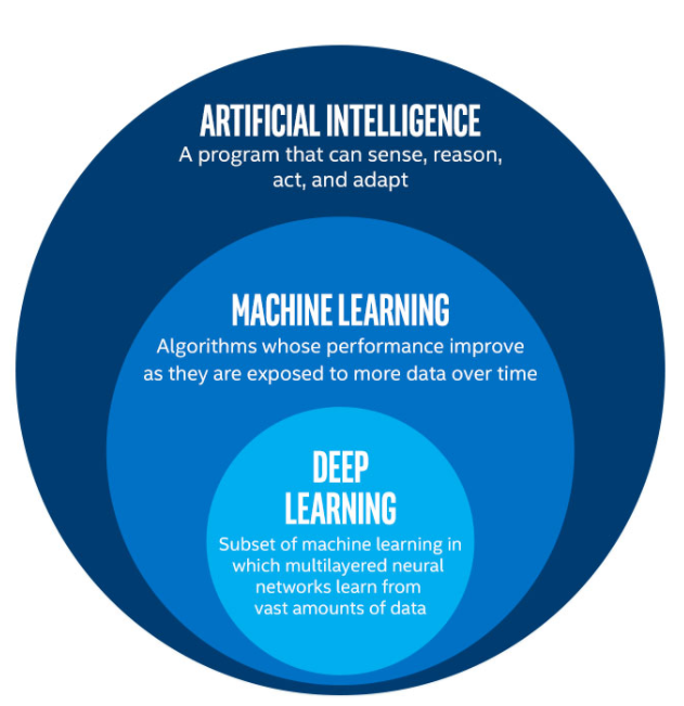
Exploring the Layers of AI: From Artificial Intelligence to Deep Learning. (Image Source: LunarTech.ai)
Deep Learning is a branch of Machine Learning, and it tries to mimic the way the human brain works and makes decisions based on neural network-based models.
In simpler terms, Deep Learning is more advanced and more complex version of traditional Machine Learning. Deep Learning Models are based on Neural Networks and they try to mimic the way humans think and make decisions.
The problem with traditional Statistical or ML methods is that they are based on specific rules and instructions. So, whenever the set of model assumptions are not satisfied, the model can have very hard time to solve the problem and perform prediction. There are also types of problems such as image recognition, and other more advanced tasks, that can’t be solved with traditional Statistical or Machine Learning models.
Here is basically where Deep Learning comes in.
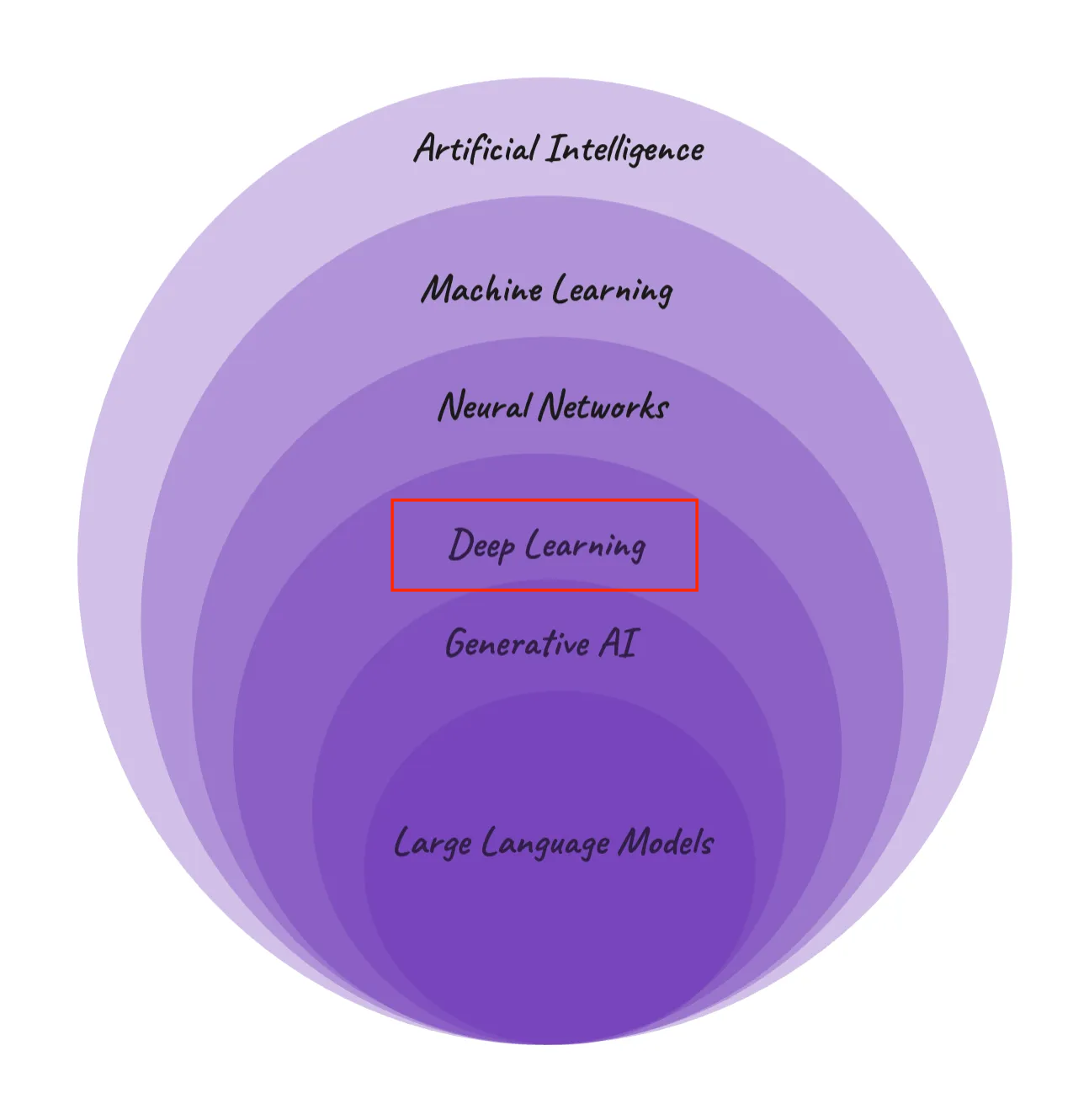
AI Hierarchy: Navigating from Broad AI Concepts to Specialized Language Models (Image Source: Medium)
Applications of Deep Learning
Here are some examples where Deep Learning is used across various industries and applications:
Healthcare
Disease Diagnosis and Prognosis: Deep learning algorithms help to analyze medical images like X-rays, MRIs, and CT scans to diagnose diseases such as cancer more accurately with computer vision models. They do this much more quickly than traditional methods. They can also predict patient outcomes by analyzing patterns in patient data.
Drug Discovery and Development: Deep Learning models help in identifying potential drug candidates and speeding up the process of drug development, significantly reducing time and costs.
Finance
Algorithmic Trading: Deep learning models are used to predict stock market trends and automate trading decisions, processing vast amounts of financial data at high speed.
Fraud Detection: Banks and financial institutions employ deep learning to detect unusual patterns indicative of fraudulent activities, thereby enhancing security and customer trust.
Automotive and Transportation
Autonomous Vehicles: Self-driving cars also use deep learning heavily to interpret sensor data, allowing them to navigate safely in complex environments, using computer vision and other methods.
Traffic Management: AI models analyze traffic patterns to optimize traffic flow and reduce congestion in cities.
Retail and E-Commerce
Personalized Shopping Experience: Deep learning algorithms help in retail and E-Commerce to analyze customer data and provide personalized product recommendations. This enhances the user experience and boosts sales.
Supply Chain Optimization: AI models forecast demand, optimize inventory, and enhance logistics operations, improving efficiency in the supply chain.
Entertainment and Media
Content Recommendation: Platforms like Netflix and Spotify use deep learning to analyze user preferences and viewing history to recommend personalized content.
Video Game Development: AI is used to create more realistic and interactive gaming environments, enhancing player experience.
Technology and Communications
Virtual Assistants: Siri, Alexa, and other virtual assistants use deep learning for natural language processing and speech recognition, making them more responsive and user-friendly.
Language Translation Services: Services like Google Translate leverage deep learning for real-time, accurate language translation, breaking down language barriers.
Manufacturing and Production
Predictive Maintenance: Deep learning models predict when machines require maintenance, reducing downtime and saving costs.
Quality Control: AI algorithms inspect and detect defects in products at high speed with greater accuracy than human inspectors.
Agriculture
- Crop Monitoring and Analysis: AI models analyze drone and satellite imagery to monitor crop health, optimize farming practices, and predict yields.
Security and Surveillance
Facial Recognition: Used for enhancing security systems, deep learning models can accurately identify individuals even in crowded environments.
Anomaly Detection: AI algorithms monitor security footage to detect unusual activities or behaviors, aiding in crime prevention.
Research and Academia
Scientific Discovery: Deep learning assists researchers in analyzing complex data, leading to discoveries in fields like astronomy, physics, and biology.
Educational Tools: AI-driven tutoring systems provide personalized learning experiences, adapting to individual student needs.
Deep Learning has drastically refined state-of-the-art speech recognition, object recognition, speech comprehension, automated translation, image recognition, and many other disciplines such as drug discovery and genomics.
Chapter 2: Foundations of Neural Networks
Now let's talk about some key characteristics and features of Neural Networks:
Layered Structure: Deep learning models, at their core, consist of multiple layers, each transforming the input data into more abstract and composite representations.
Feature Hierarchy: Simple features (like edges in image recognition) recombine from one layer to the next, to form more complex features (like objects or shapes).
End-to-End Learning: DL models perform tasks from raw data to final categories or decisions, often improving with the amount of data provided. So, large data plays ket role for Deep Learning.
Here are the core components of Deep Learning models:
Neurons
These are the basic building blocks of neural networks that receive inputs and pass on their output to the next layer after applying an activation function (more on this in the following chapters).
Weights and Biases
Parameters of the neural network that are adjusted through the learning process to help the model make accurate predictions. These are the values that the optimization algorithm should continuously optimize ideally in short amount of time to reach the most optimal and accurate model (for example, commonly referenced by w_ij and b_ij ).
Bias Term: In practice, a bias term ( b ) is often added to the input-weight product sum before applying the activation function. This is a term that enables the neuron to shift the activation function to the left or right, which can be crucial for learning complex patterns.
Learning Process: Weights are adjusted during the network's training phase. Through a process often involving gradient descent, the network iteratively updates the weights to minimize the difference between its output and the target values.
Context of Use: This neuron could be part of a larger network, consisting of multiple layers. Neural networks are employed to tackle a vast array of problems, from image and speech recognition to predicting stock market trends.
Mathematical Notation Correction: The equation provided in the text uses the symbol ( \phi ), which is unconventional in this context. Typically, a simple summation ( \sum ) is used to denote the aggregation of the weighted inputs, followed by the activation function ( f ), as in
$$f\left(\sum_{i=1}^{n} W_ix_i + b\right)$$
Activation Functions
Functions that introduce non-linear properties to the network, allowing it to learn complex data patterns. Thanks to activation functions, instead of acting as of all input signals or hidden units are equally important, activation functions help to transform the these values, which results instead of linear type of model to a non-linear much more flexible model.
Each neuron in a hidden layer transforms inputs from the previous layer with a weighted sum followed by a non-linear activation function (this is what differentiates your non-linear flexible neural network from common linear regression). The outputs of these neutrons are then passed on to the next layer and the next one, and so on, until the final layer is achieved.
We will discuss activation functions in detail in this handbook, along with the examples of 4 most popular activation functions to make this very clear as it's very important concept and is crucial part of learning process in neural networks.
This process of inputs going through hidden layers using activation function(s) and resulting in an output is known as forward propagation.
Architecture of Neural Networks
Neural network usually have three types of layers: input layers, hidden layers, and output layers. Let's learn a bit more about each of these now.
We'll use our house price prediction example to learn more about these layers. Below you can see the figure visualizing a simple neural network architetcure which we will unpack layer by layer.
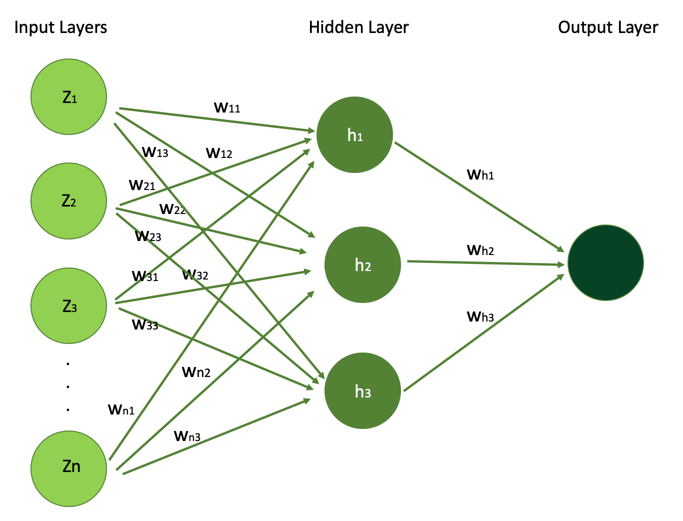
Simple Neural Network Architecture: Inputs, Weights, and Outputs Explained (Image Source: LunarTech.ai)
Input layers
Input layers are the initial layers where the data is. They contain the features that your model takes in as input to then train your model.
This is where the neural network receives its input data. Each neuron in the input layer of your neural network represents a feature of the input data. If you have two features, you will have two input layers.
Below is the visualization of architecture of simple Neural Network, with N input features (N input signals) which you can see in the input layer. You can also see the single hidden layer with 3 hidden units h1,h2, and h3 and the output layer.
Let's start with Input Layer and understand what are those Z1, Z2, ... , Zn features.
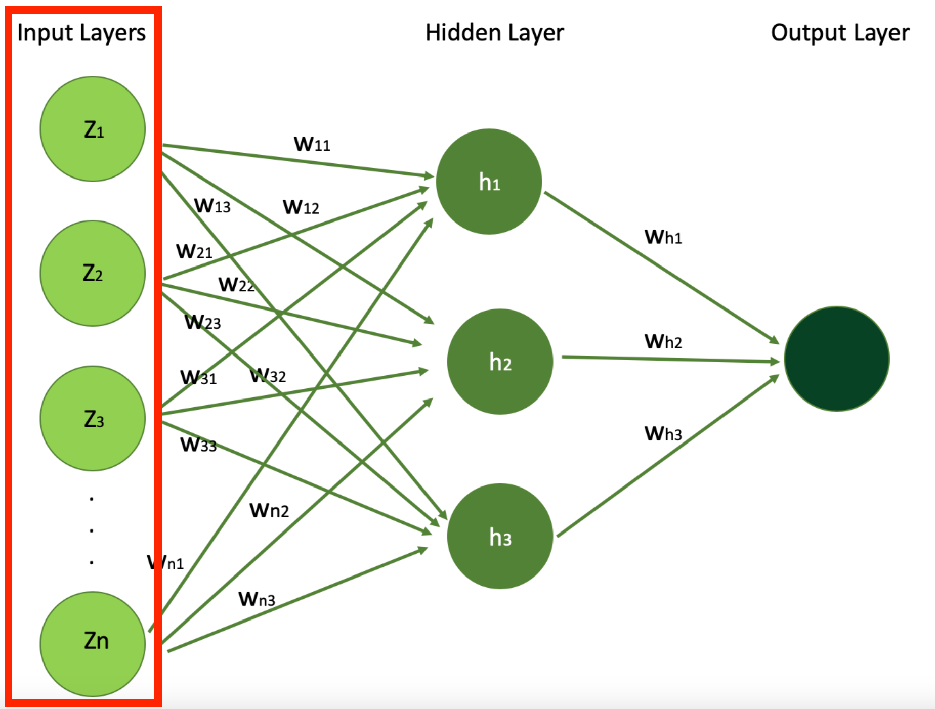
Simple Neural Network Architecture Highlighting the Input Layers (Image Source: LunarTech.ai)
In our example of using neural networks for predicting a house's price, the input layer will take house features such as the number of bedrooms, age of the house, proximity to the ocean, or whether there's a swimming pool, in order to learn about the house. This is what will be given to the input layer of the neural network. Each of these features serves as an input neuron, providing the model with essential data.
But then there's the question of how much each of these features should contribute to the learning process. Are they all equally important, or some are more important and should contribute more to the estimation of the price?
The answer to this question lies in what we are calling "weights" that we defined earlier along with bias factors.
In the figure above, each neuron gets weight w_ij where i is the input neuron index and j is the index of the hidden unit they contribute in the Hidden Layer. So, for example w_11, w_12, w_13 describe how much feature 1 is important for learning about the house for hidden unit h1, h2, and h3 respectively.
Keep these weight parameter in mind as they are one of the most important parts of a neural network. They are the importance weights that the neural network will be updating during training process, in order to optimize the learning process.
Hidden layers
Hidden layers are the middle part of your model where learning happens. They come right after Input Layers. You can have from one to many hidden layers.
Let's simplify this concept by looking at our simple neural network along with our house price example.
Below, I highlighted the Hidden Layer in our simply neural network whose architecture we saw earlier, which you can think of as a very important part in your neural network to extract patterns and relationships from the data that are not immediately apparent from the first view.
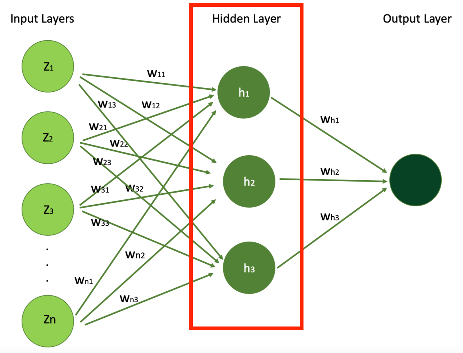
Simple Neural Network Architecture Highlighting the Hidden Layer (Image Source: LunarTech.ai)
In our example of estimating a house's price with a neural network, the hidden layers play a crucial role in processing and interpreting the information received from the input layer, like the house features we just mentioned above.
These layers consist of neurons that apply weights and biases to the input features – like house age, number of bedrooms, proximity to the ocean, and the presence of a swimming pool – to extract patterns and relationships that are not immediately apparent.
In this context, hidden layers might learn complex interdependencies between house features, such as how the combination of a prime location, house age and modern amenities significantly boosts the price of the house.
They act as the neural network's computational engine, transforming raw data into insights that lead to an accurate estimation of a house's market value. Through training, the hidden layers adjust these weights and biases (parameters) to minimize models prediction errors, gradually improving the model's accuracy in estimating house prices.
These layers perform the majority of the computation through their interconnected neurons. In this simple example, we've got only 1 hidden layer, and 3 hidden units (for example, another hyperparameter to optimize during your learning using techniques such as Random Search CV or others).
But in real world problems, neural networks are much deeper and your number of hidden layers, with the weights and bias parameters, can exceed billions with many hidden layers.
Output layer
Output layers are the final component of a neural network – the final layer which provides the output of the neural network after all the transformations into output for specific single task. This output can be single value (in regression case for example) or a vector (like in large language models were we produce vector of probabilities, or embeddings).
An output layer can be a class label for a classification model, a continuous numeric value for regression model, or even a vector of numbers, depending on the task.
Hidden layers in neural network are where the actual learning happens, where the deep learning network learns from the data by extracting and transforming the provided features.
As the data goes deeper into the network, the features become more abstract and more composite, with each layer building on the previous layers output/values. The depth and the width (number of neurons) of hidden layers are key factors in the network’s capacity to learn complex patterns. Below is the digram we saw before showcasing the architecture of simple neural networks.
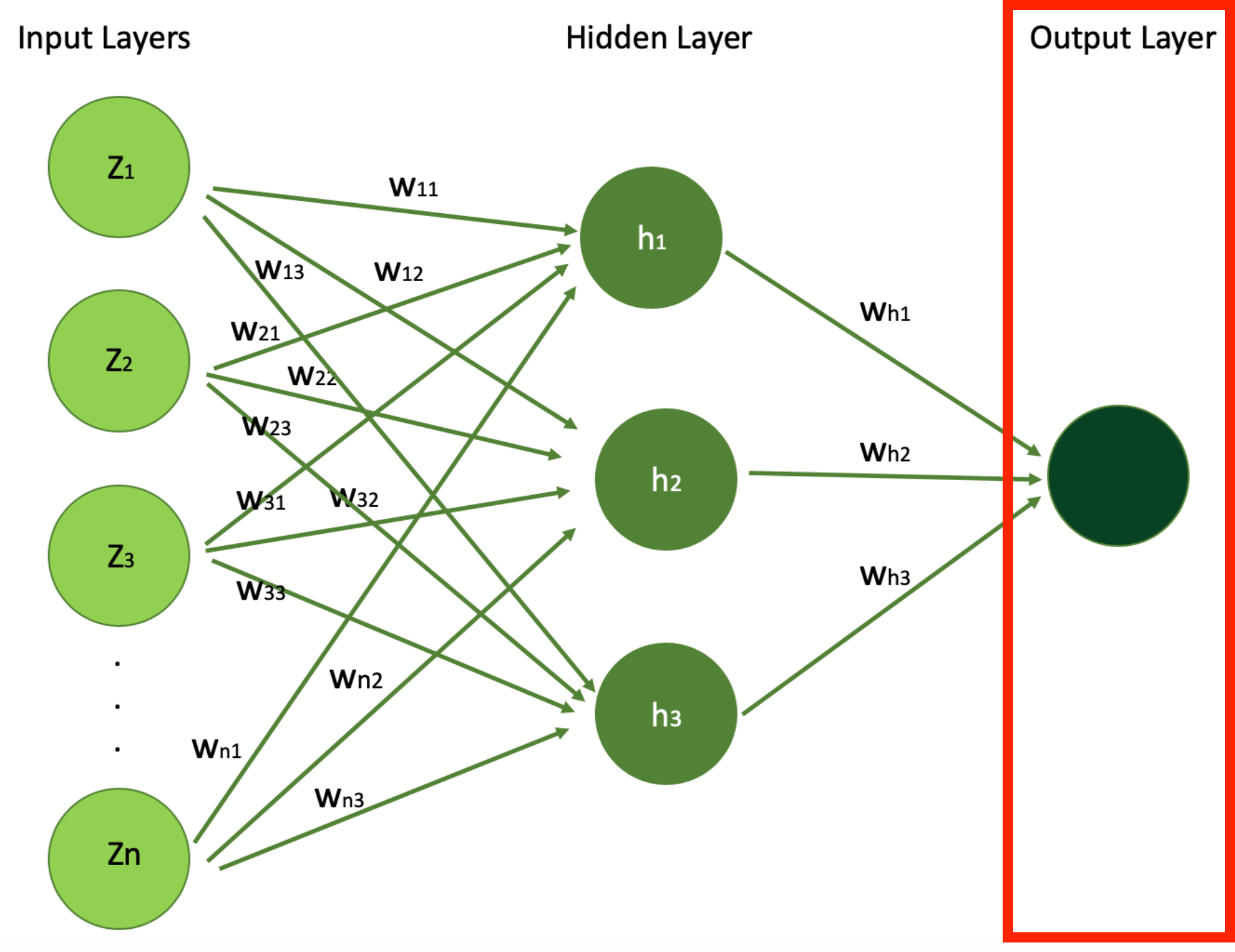
Simple Neural Network Architecture Highlighting the Output (Image Source: LunarTech.ai)
In our example of house price prediction, the culmination of the learning process is represented by the output layer, which represents our final goal: the predicted house price.
Once the input features – like the number of bedrooms, the age of the house, distance to the ocean, and whether there's a swimming pool – are fed into the neural network, they travel through one or more hidden layers of neural network. It's within these hidden layers that neural network discovers complex patterns and interconnections within the data.
Finally, this processed information reaches the output layer, where the model consolidates all its findings and produces the final results or predictions, in this case the house price.
So, the output layer consolidates all the insights gained. These transformations are applied throughout the hidden layers to produce a single value: the predicted price of the house (often referred to by Y^, pronounced "Y hat").
This prediction is the neural network's estimation of the house's market value, based on its learned understanding of how different features of the house affect the house price. It demonstrates the network's ability to synthesize complex data into actionable insights, in this case, producing an accurate price prediction, through its optimized model.
Activation functions
Activation functions introduce non-linear properties to the neural network model, which enables the model to learn more complex patterns.
Without non-linearity, your deep network would behave just like a single-layer perceptron, which can only learn linear separable functions. Activation functions define how the neurons should be activated – hence the name activation function.
Activation functions serve as the bridge between the input signals received by the network and the output it generates. These functions determine how the weighted sum of input neurons – each representing a specific feature like the number of bedrooms, house age, proximity to the ocean, and presence of a swimming pool – should be transformed or "activated" to contribute to the network's learning process.
Activation functions are an extremely important part of training Neural Nets. When the net consists of Hidden Layers and Output Layers, you need to pick an activation function for both of them (different activation functions may be used in different parts of the model). The choice of activation function has a huge impact on the neural networks’ performance and capability.
Each of the incoming signals or connections are dynamically strengthened or weakened based on how often they are used (this is how we learn new ideas and concepts). It is the strength of each connection that determines the contribution of the input to the neurons’ output.
After being weighted by the strength of their respective signals, the inputs are summed together in the cell body. This is then transformed into a new signal that’s transmitted or propagated along the cells’ axon and sent off to other neurons. This functional work of activation function can mathematically be represented as follows:
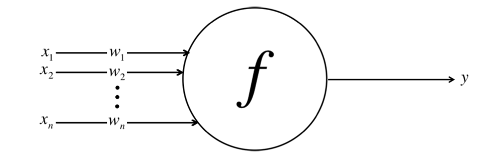
Neuron Activation: Transforming Weighted Inputs into Outputs (Image Source: LunarTech.ai)
Here we have inputs x1, x2, ...xn and their corresponding weights w1, w2, ... wn, and we aggregate them into single value of Y by using activation function f.
This figure is a simplified version of a neuron within an artificial neural network. Each input ( X_i ) is associated with a corresponding weight ( W_i ), and these products are aggregated to compute the output ( Y ) of the neuron. The X_i is the input value of signal i (like the number of bedrooms of the house, as a feature describing the house). Its importance weight by w_i corresponds to each X_i, so the sum of all these weighted input values can be expressed as follows:
$$\phi\left(\sum_{i=1}^{m} w_i x_i\right)$$
In this equation, phi represents the function we use to join signals from different input neurons into one value. This function is called the Activation Function.
Each synapse gets assigned a weight, an importance value. These weights and biases form the cornerstone of how Neural Networks learn. These weights and biases determine whether the signals get passed along or not, or to what extent each signal gets passed along.
In the context of predicting house prices, after the input features are weighted according to their relevance learned through training, the activation function comes into play. It takes this weighted sum of inputs and applies a specific mathematical operation to produce an activation score.
This score is a single value that efficiently represents the aggregated input information. It enables the network to make complex decisions or predictions based on the input data it receives.
Essentially, activation functions are the mechanism through which neural networks convert an input's weighted sum into an output that makes sense in the context of the specific problem being solved (like estimating a house's price here). They allow the network to learn non-linear relationships between features and outcomes, enabling the accurate prediction of a house's market value from its characteristics.
The modern default or most popular activation function for hidden layers is the Rectifier Linear Unit (ReLU) or Softmax function, mainly for accuracy and performance reasons. For the output layer, the activation function is mainly chosen based on the format of the predictions (probability, scaler, and so on).
Whenever you are considering any activation function, be aware of the Vanishing Gradient Problem (we will revisit this topic later). This happens when gradients are too small or too large, they can make the learning process difficult.
Some activation functions like sigmoid or tanh can cause vanishing gradients in deep networks while some of them can help mitigate this issue.
Let's look at a few other kinds of activation functions now, and when/how they're useful.
Linear Activation Function
A Linear Activation Function can be expressed as follows:
$$f(z) = z$$
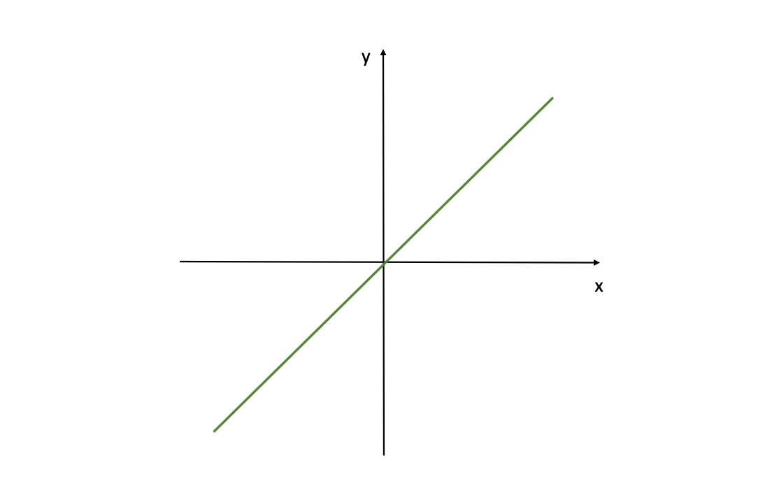
Linear Activation Function (Image Source: LunarTech.ai)
This grapgh shows a linear activation function for a neural network, defined by f(z)=z. Where z is the input (called Z-scores as we mentioned before) for the activation function f( ). This means the output is directly proportional to the input.
Linear Activation Functions are the simplest activation functions, and they're relatively easy to compute. But they have an important limitation: NNs with only linear neurons can be expressed as a network with no hidden layers – but the hidden layers in NNs are what enables them to learn important features from input signals.
So, in order to learn complex patterns from complex problems, we need more advanced Activation Functions rather than Linear Functions.
You can use a linear function, for instance, in the last output layer when the plain outcome is good enough for you and you don’t want any transformation. But 99% of the time this activation function is useless in Deep Learning.
Sigmoid Activation Function
One of the most popular activation functions is the Sigmoid Activation Function, which can be expressed as follows:
$$f(z) = \frac{1}{1 + e^{-z}}$$
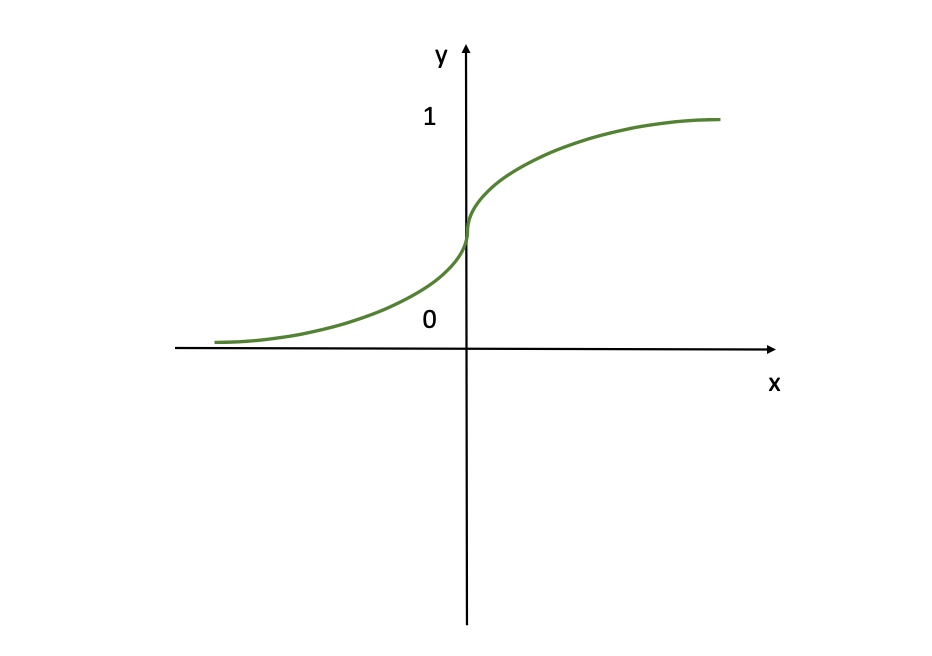
Sigmoid Activation Function (Image Source: LunarTech.ai)
In this figure the sigmoid activation function is visualised, which is a smooth, S-shaped curve commonly used in neural networks. If you are familiar with Logistic Regression, then this function will seem familiar to you as well. This function transforms all input values to values in the range of (0,1) which is very convenient when you want the model to provide output in the form of probabilities or a %.
Basically, when the logit is very small, the output of a logistic neuron is very close to 0. When the logit is very large, the output of the logistic neuron is closer to 1. In-between these two extreme values, the neuron assumes an S-shape. This S-shape of the curve also helps to differentiate between outputs that are close to 0 or close to 1, providing a clear decision boundary.
You'll often use the Sigmoid Activation Function in the output layer, as it’s ideal for the cases when the goal is to get a value from the model as output between 0 and 1 (a probability for instance). So, if you have a classification problem, definitely consider this activation function.
But keep in mind that this activation is very intensive and a large amount of neurons will be activated. This is also why, for the hidden units, the Sigmoid activation is not the best option, as it sets large values to the bounds of 0 and 1, causing quickly parameters stay constant → no gradients (used to update the weights and bias factors).
This is the infamous Vanishing Gradient Problem (more on this in the upcoming chapters). This results in the model being unable to accurately learn from the data and produce accurate predictions.
ReLU (Rectifier Linear Unit)
A different type of nonlinear relationship is uncovered when using the Restricted Linear Unit (ReLU) . This activation function is less strict and works great when your focus is on positive values.
The ReLU activation function activates the neurons that have positive values but deactivates the negative values, unlike the Sigmoid function which activates almost all neurons. This activation function can be expressed as follows:
$$f(z) = \begin{cases} 0 & \text{if } z < 0 \\ z & \text{if } z \geq 0 \end{cases}$$
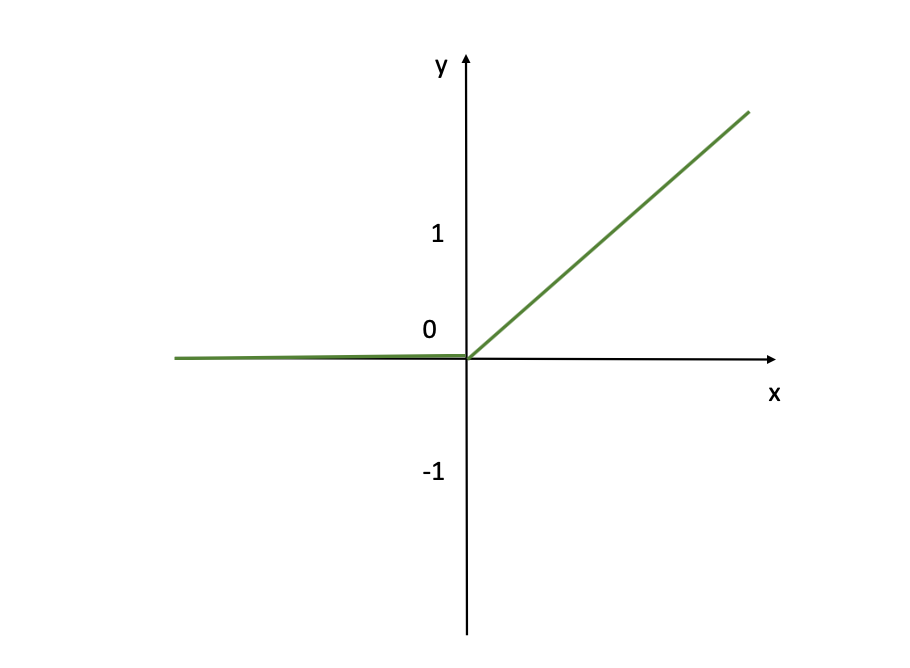
ReLU Activation Function (Image Source: LunarTech.ai)
As you can see above from this visualization, the ReLU activation function doesn’t activate at all the input neurons with negative values (you can see that for the x's which are negative, corresponding Y-axis value is 0). While for positiove inputs x, the activation function returns the exact value x (Y=X linear line as you see from the figure). But it is still a good default choice for hidden layers. It is computationally efficient and reduces the likelihood of vanishing gradients during training, especially for deep networks.
Leaky ReLU Activation Function
While ReLU doesn’t activate input neurons with negative values, the Leaky ReLU does account for these negative input values. It learns from it though with a lower rate equal to 0.01.
This activation function can be expressed as follows:
$$f(z) = \begin{cases} 0.01z & \text{if } z < 0 \\ z & \text{if } z \geq 0 \end{cases}$$
So, the Leaky ReLU allows for a small or non-zero gradient when the input value is saturated and not active.
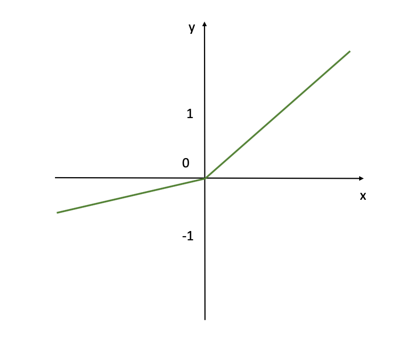
Leaky ReLU Activation Function (Image Source: LunarTech.ai)
This visualization shows the Leaky ReLU activation function commonly used neural networks especially for the hidden layers and where negative activations is acceptable. Unlike the standard ReLU, which gives an output of zero for any negative input, Leaky ReLU allows a small, non-zero output for negative inputs.
Like ReLU, Leaky ReLU is also a good default choice for hidden layers. It is computationally efficient and reduces the likelihood of vanishing gradients during training, especially for deep networks with multiple hidden layers.We will talk more on these and previous activations functions when discussing the Vanishing Gradient Problem, and if you want bit more details and the concept to be explained in tutorial - check out the resources below.
Hyperbolic Tangent (Tanh) Activation Function
Hyperbolic Tangent activation function is often referred to simply as the Tanh function. It's very similar to the Sigmoid activation function. It even has the same S-shape representation.
This function takes any real value as input value and outputs a value in the range -1 to 1. This activation function can be expressed as follows:
$$f(z) = \tanh(z) = \frac{e^z - e^{-z}}{e^z + e^{-z}}$$
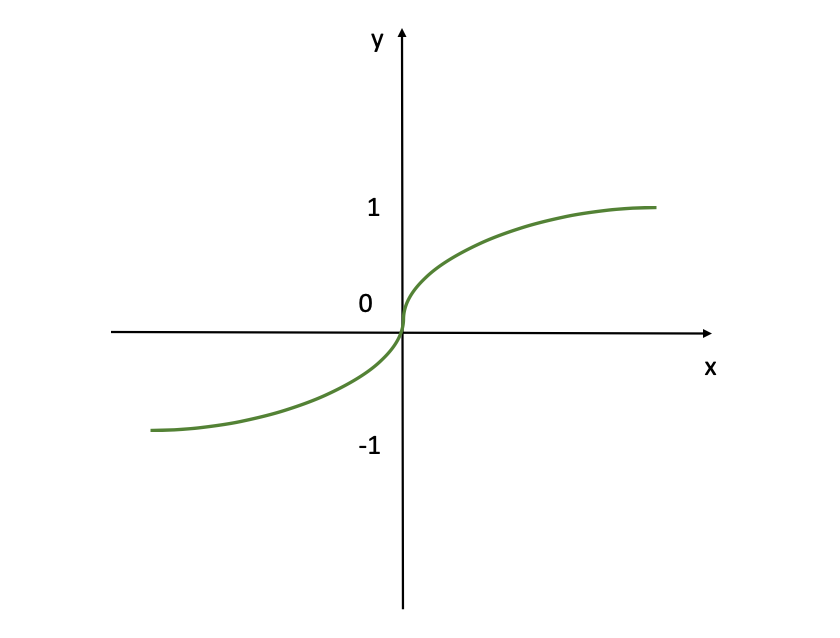
Tanh Activation Function (Image Source: LunarTech.ai)
The figure shows the tanh (hyperbolic tangent) activation function. So, this function outputs values ranging from -1 to 1, providing a normalized output that can help with the convergence of neural networks during training. It's similar to the sigmoid function but it is adjusted to allow for negative outputs, which can be beneficial for certain types of neural networks where the mean of the outputs needs to be centered around zero.
Note - if you want to get more details about these activation functions, check out this tutorial where I cover this concept in further detail at "What is an Activation Function" and "How to Solve the Vanishing Gradient Problem".
Again, the current default or most popular activation function for hidden layers is the Rectifier Linear Unit (ReLU) or Softmax function, mainly for accuracy/performance reasons. For the output layer, the activation function is mainly chosen based on the format of the predictions (probability, scaler, and so on).
Chapter 3: How to Train Neural Networks
Training neural networks is a systematic process that involves two main processes, done repeatedly, named forward and backward passes.
First the data goes through the Forward Pass until the output. Then it is followed by a backward pass. The idea behind this process is to go through the network on multiple occasions to adjust the weights and minimize the loss or cost functions.
To get a better understanding, we will look into a simple Neural Network where we have 3 input signals, and just a single hidden layer that has 4 hidden units. This can be visualized as follows:
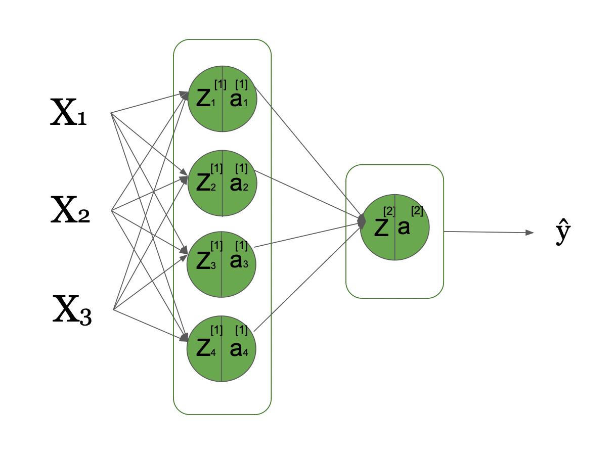
From Input Layer through Hidden Layers to Prediction (Image Source: LunarTech.ai)
Here you can see that we have 3 input signals in our input layer, 1 hidden layer with 4 hidden units, and 1 output layer. This is a computational graph visualizing this basic neural network and how the information flows from the left, initial inputs to the right, all the way down to the predicted Y^ (Y hat), after going through multiple transformations.

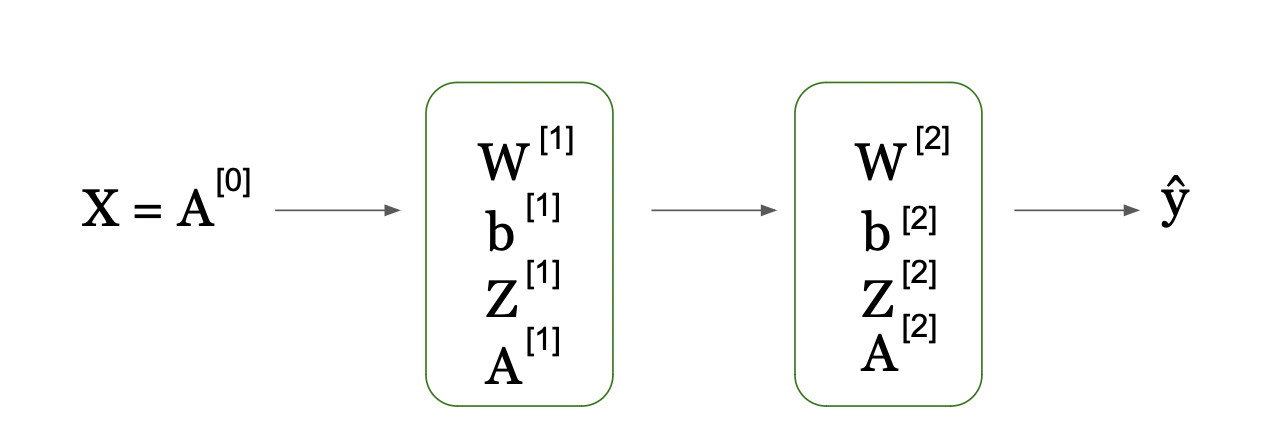
Forward and Backward Propagation in Neural Networks (Image Source: LunarTech.ai)
Now, let's look into this figure that showcases the high level idea of flow of information.
We go from input X (which we define by A[0] as the initial activations)
Then per step (indexed by [1]) we take the weights matrix (W[1] and bias vector b[1]) and compute the Z scores (Z[1])
Then we apply the activation function to get activation scores (A[1]) at level [1]. This happens at time step 1, which is in our example hidden layer 1.
As we get a single layer, the next step is the output layer, where the information from the previous layer (A[1]) is used to compute the new Z[2] scores by combining the input A[1] from the previous layer and with W[2] / b[2] from this layer. We then apply another activation layer (our output layer activation function) on the just computed Z[2] to compute the A[2].
As the A[2] is in the output layer, this gives us our prediction, Y_hat. This is the Forward Pass or Forward Propagation.
Next you can see in the second part of the figure, we go from Y_hat to all these terms that are kind of the same as in forward pass but with one crucial difference: they all have "d" in front of them, which refers to the "derivative".
So, after the Y_hat is produced, we get our predictions, and the network is able to compare the Y_hat (predicted values of response variable y, in our example house price) to the true house prices Y and obtain the Loss function.
If you want to learn more about Loss Functions, check out here or this tutorial.
Then, the network computes the derivative of loss function with regard to activations A and Z score (dA and dZ). Then it uses these to compute the gradients/derivatives with regard to the weights W and biases b (dW and db).
This also happens per layer and in a sequential way, but as you can see from the arrow in the figure above, this time it happens backwards from right to left unlike in forward propagation.
This is also why we refer this process as backpropagation. The gradients of layer 2 contribute to the calculation of the gradients in layer 1, as you can also see from the graph.
Forward Pass
Forward propagation is the process of feeding input data through a neural network to generate an output. We will define the input data by X which contains 3 features X1, X2, X3 which can be described mathematically as follows:
zi=ωTxi+b
⇓
y^i=ai=σ(zi)
⇓
l(ai,yi)
Where in these equations we are moving from input x_i in our simple neural network, to the calculation of loss.
Let's unpack them:
Step 1: Each neuron in subsequent layers calculates a weighted sum of its inputs (x^i) plus a bias term b. We call this a score z^i. The inputs are the outputs from the previous layer’s neurons, and the weights as well as the bias are the parameters that neural network is aiming to learn and estimate.
Step 2: Then using an activation function, which we denote by the Greek letter delta, the network transforms the Z scores to a new value which we define by a^i. Note that the activation value at the initial pass when we are at the initial layer in the network (layer 0) is equal to x^i. This is then the predicted value in that specific pass.
To be more accurate, let’s make our notation a bit more complicated. We'll define each score in the first hidden layer, layer [1], per unit (as we have 4 units in this hidden unit) and generalize this per hidden unit i:
zi[1]=(ωi[1])Tx+(bi[1])Tfor i=1,2,3,4
ai[1]=σ(zi[1])
Let’s now rewrite this using Linear Algebra and specifically matrix and vector operations:
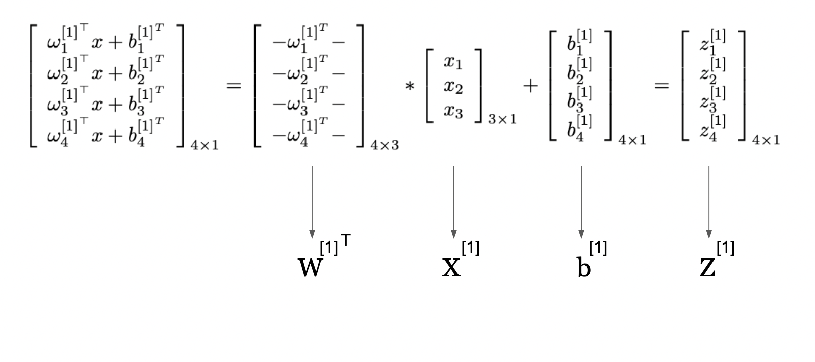
Matrix Operations in Neural Network Computations (Image Source: LunarTech.ai)
This image presents a way to represent the computations in a neural network layer using matrix operations from Linear Algebra. It shows how individual computations for each neuron in a layer can be compactly expressed and performed simultaneously through using matrix multiplication and summation.
The matrix labeled W^[1] contains the weights applied to the inputs for each neuron in the first hidden layer. The vector X[1] is the input to the layer. By multiplying the weight matrix with the input vector and then adding the bias vector b[1], we get the vector Z[1], which we refered as Z-score previously too and represents the weighted sum of inputs plus the bias for each neuron.
This compact form allows us to use efficient linear algebra routines to compute the outputs of all neurons in the layer at once.
This approach is fundamental in neural networks as it enables the processing of inputs through multiple layers efficiently, allowing neural networks to scale to large numbers of neurons and complex architectures.
So, here we go from unit level to representing the transformations in our simple neural networks by using Matrix multiplication and summations from Linear Algebra.
First Layer Activation
Now, let's look into this equation that showcases the high level idea of flow of information when we go from input X[1] (which we define by A[0] as the initial activations) then per step (indexed by [1]) we take the weights matrix (W[1] and bias vector b[1]) and compute the Z scores (Z[1]). Then we apply activation function of layer 1, g[1] to get activation scores (A[1]) at level [1]. This happens at time step 1, which is in our example hidden layer 1.
Second (Output) Layer Activation
As we get a single layer, next step is the output layer, where the information from the previous layer (A[1]) is used to compute the new Z[2] scores by combining the input A[1] from previous layer and with W[2] / b[2] from this layer. We then apply another activation function g[2] (our output layer activation function) on just computed Z[2] to compute the A[2].
After the activation function has been applied, it can then be fed into the next layer of the network if there is one, or directly to the output layer if this is a single hidden layer network. As in our case, layer 2 is our output layer, we are ready to go to Y_hat, our predictions.
Sequential Data Flow Through Neural Network Layers (Image Source: LunarTech.ai)
This image shows a way to represent the computations in a neural network layer using matrix operations. It shows how individual computations for each neuron in a layer of neural network can be compactly expressed, performed simultaneously through matrix multiplication and addition.
Here, the matrix labeled W[1] contains the weights applied to the inputs for each neuron in the first hidden layer. The vector X[1] is the input to this layer. By multiplying the weight matrix by the input vector and then adding the bias vector b[1], we get vector Z[1], which represents the weighted sum of inputs plus the bias for each neuron.
This compact form allows us to use efficient linear algebra routines to compute the outputs of all neurons in the layer at once. The resulting vector Z[1] is then passed through an activation function (not shown in this part of the image), which performs a non-linear transformation on each element, resulting in the final output of the layer.
This approach is fundamental in neural networks as it enables the processing of inputs through multiple layers efficiently, allowing neural networks to scale to large numbers of neurons and complex architectures.
Computing the Loss Function
As the A[2] is in the output layer, this gives us our prediction, Y_hat. After the Y_hat is produced, we got our predictions, and the network is able to compare the Y_hat (predicted values of response variable y, in our example house price) to the true house prices Y, and obtain the Loss function J. The total loss can be calculated as follows:
where log() is the logarithm used to compute this loss function.
Backward Pass
Backpropagation is a crucial part of the training process of a neural network. Combined with optimization algorithms like Gradient Descent (GD), Stochastic Gradient Descent (SGD), or Adam, they perform the Backward Pass.
Backpropogation is an efficient algorithm for computing the gradient of the cost (loss) function (J) with respect to each parameter (weight & bias) in the network.
So, to be clear, backpropagation is the actual process of calculating the gradients in the model, and then Gradient Descent is the algorithm that takes the gradients as input and updates the parameters.
When we compute the gradients and use them to update the parameters in the model, this helps us update the parameters and direct them towards more correct direction towards finding the global optimum to minimize. This helps further minimize the loss function and improve prediction accuracy of the model.
In each pass, after forward propagation is completed, the gradients should be obtained. Then we use them to obtain the model parameters, such as the weight and the bias parameters.
Let’s look at an example of the gradient calculations for backpropagation in a neural network that we saw in Forward Propagation with a single hidden layer and 4 hidden units.
Backpropagation always starts from the end, so let’s visualize it to help you understand this process better:
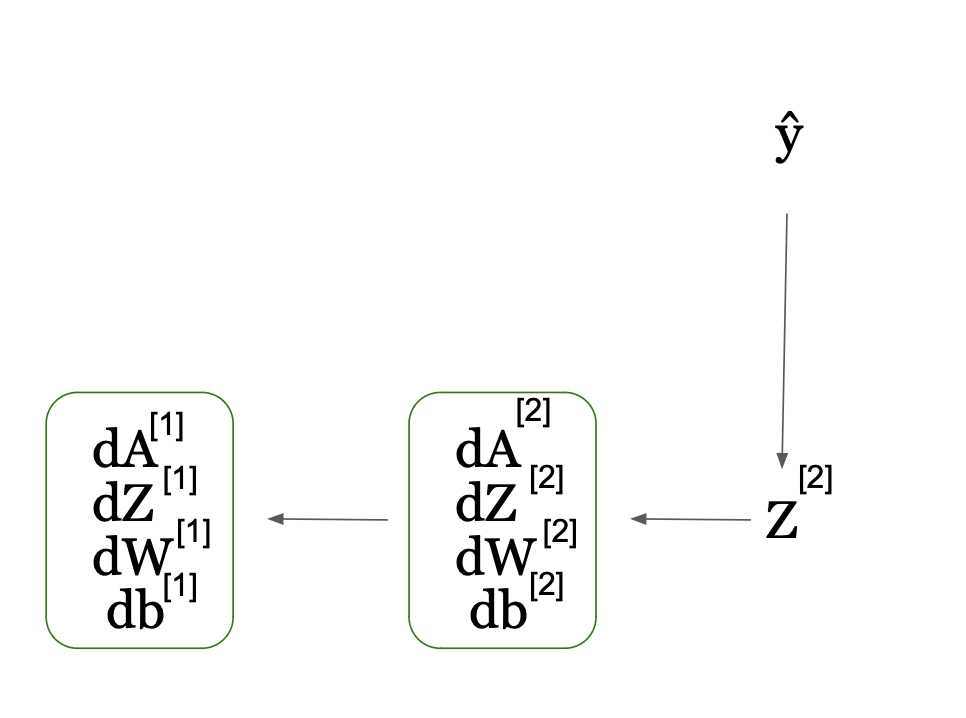
Backpropagation Process in Neural Networks: Calculating Gradients (Image Source: LunarTech.ai)
In this figure, the network computes the derivative of the loss function with regard to activations A and Z score (dA and dZ). It then uses these to compute the gradients/derivatives with regard to weights W and biases b (dW and db). This also happens per layer and in sequential way, but as you can see from the arrow in the figure, this time it happens backwards from right to left unlike in forward propagation.
This is also why we refer this process as backpropagation. The gradients of layer 2 contribute to the calculation of the gradients in layer 1 as you can also see from the graph.
So, the idea is that we calculate the gradients with respect to the activation (dA[2]), then with respect to the pre-activation (dZ[2]), and with respect the weights (dW[2]) and bias (db[2]) of the output layer, assuming we have a cost function J after we have computed the Y^. Make sure to always cache the Z[i] as they are needed in this process.
Mathematically, the gradients can be calculated using the common differentiation rules including obtaining the derivative of the logarithm, and using Sum Rule and Chain Rules. The first gradient dA[2] can be expressed as follows:
The next gradient we need to compute is the gradient of the cost function with respect to Z[2], that is dZ[2].
We know the following:
A[2]=σ(Z[2])
dJdA[2]=dA[2]dZ[2]
dA[2]dZ[2]=σ′(Z[2])
So, A[2] = σ(Z[2]), we can then use these derivatives of the sigmoid function σ'(Z[2]) = σ(Z[2]) * (1 - σ(Z[2])). This can be derived mathematically as follows:
$$\begin{align*} \frac{dZ^{[2]}}{dJ} &= \frac{dJ}{dZ^{[2]}} \\ \downarrow \\ \frac{dZ^{[2]}}{dJ} &= \frac{dJ}{dA^{[2]}} \cdot \frac{dA^{[2]}}{dZ^{[2]}} \quad \text{using chain rule} \\ \downarrow \\ \frac{dZ^{[2]}}{dJ} &= dA^{[2]} \cdot \sigma'(Z^{[2]}) \\ \downarrow \\ \frac{dZ^{[2]}}{dJ} &= dA^{[2]} \cdot A^{[2]} \cdot (1 - A^{[2]}) \end{align*}$$
$$\begin{align*} \sigma(Z^{[2]}) &= \frac{1}{1 - e^{Z^{[2]}}} = (1 - e^{-Z^{[2]}})^{-1} \\ \downarrow \\ \sigma'(Z^{[2]}) &= \frac{d\sigma(Z^{[2]})}{dZ^{[2]}} \\ \downarrow \\ \sigma'(Z^{[2]}) &= -\frac{-1}{(1 - e^{Z^{[2]}})^2} \cdot (-1) \cdot e^{Z^{[2]}} \\ \downarrow \\ \sigma'(Z^{[2]}) &= \frac{1}{1 - e^{Z^{[2]}}} \cdot \frac{e^{Z^{[2]}}}{1 - e^{Z^{[2]}}} \\ \downarrow \\ \sigma'(Z^{[2]}) &= \sigma(Z^{[2]}) \cdot (1 - \sigma(Z^{[2]})) = A^{[2]} \cdot (1 - A^{[2]}) \end{align*}$$
Now when we know the how and the why behind the calculation of the gradient with regard to the Z score, we can calculate the gradient with regard to the weight W. This is very important for updating the weight parameter value (for example, direction).
$$\begin{align*} Z^{[2]} &= W^{[2]T} \cdot A^{[1]} + b^{[2]} \\ \downarrow \\ \frac{db^{[2]}}{dZ^{[2]}} &= \frac{dJ}{dZ^{[2]}} \cdot \frac{dZ^{[2]}}{db^{[2]}} \quad \text{using chain rule} \\ \downarrow \\ db^{[2]} &= dZ^{[2]} \cdot 1 + 0 \quad \text{using constant rule} \\ \downarrow \\ db^{[2]} &= dZ^{[2]} \end{align*}$$
Now in this step, the only thing remaining is to calculate the gradient with regard to the bias, our second parameter b, in the hidden layer, layer 2.
$$\begin{align*} Z^{[2]} = W^{[2]T} \cdot A^{[1]} + b^{[2]} \\ \frac{db^{[2]}}{dJ} = \frac{dJ}{dZ^{[2]}} \cdot \frac{dZ^{[2]}}{db^{[2]}} \quad \text{using chain rule} \\ db^{[2]} = dZ^{[2]} \cdot 1 + 0 \quad \text{using constant rule} \\ db^{[2]} = dZ^{[2]} \end{align*}$$
Since b[2] is a bias term, its derivative is simply the sum of the gradients dZ[2] across all the training examples (which, in a vectorized implementation, is often done by summing dZ[2] across the m observations).
Once backpropogation is done, next step is to use these gradients as input for optimization algorithm like GD, SGD, or others to find out how the parameters should be updated.
So, we are finally ready to update the Weight and Bias parameters of the model in this pass.
Here is an example using the GD algorithm:
$$W^{[2]} = W^{[2]} - \eta \cdot dW^{[2]}$$
$$b^{[2]} = b^{[2]} - \eta \cdot db^{[2]}$$
Here the η represents the learning parameter assuming the simple GD optimization's algorithm (more on the optimization algorithms in later chapters).
In the next section, we will go into more detail about how you can use various optimization algorithms to train Deep Learning models.
Chapter 4: Optimization Algorithms in AI
Once the gradient is computed via backpropagation, the next step is to use an optimization algorithm to adjust the weights to minimize the cost function.
To be clear, the optimization algorithm takes as input the calculated gradients and uses this to update model parameters.
These are the most popular optimization algorithms used when training Neural Networks:
Gradient Descent (GD)
Stochastic Gradient Descent (SGD)
SGD with Momentum
RMSProp
Adam Optimizer
Knowing the fundamentals of the Deep Learning models and learning how to train those models is definitely a big part of Deep Learning. If you have read so far and the math hasn’t made you tired, congratulations! You have grasped some challenging topics. But that’s only part of the job.
In order to use your Deep Learning model to solve actual problems, you'll need to optimize it after you have established its baseline. That is, you need to optimize the set of parameters in your Machine Learning model to find the set of optimal parameters that result in the best performing model (all things being equal).
So, to optimize or to tune your Machine Learning model, you need to perform hyperparameter optimization. By finding the optimal combination of hyperparameter values, we can decrease the errors the model produces and build the most accurate neural network.
A model's hyperparameter is a constant in the model. It’s external to the model, and its value cannot be estimated from data (but rather should be specified in advance before the model is trained). For instance, weights and bias parameters in neural network are parameters we want to optimize.
NOTE: As optimization algorithms are used across all neural networks, I thought it will be useful to provide you the Python code which you can implement to perform neural network optimization manually.
Just keep in mind that this is not what you will do in practice, as there are libraries for this purpose. Still, seeing the Python code will help you to understand the actual workings of these algorithms like GD, SGD, SGD with Momentum, Adam, AdamW much better.
I will provide you the formulas, explanations, as well as the Python code so you can see that is the Python code behind the actual functions of the libraries that implement these optimization algorithms.
Gradient Descent (GD)
The Batch Gradient Descent algorithm (often just referred to as Gradient Descent or GD), computes the gradient of the Loss Function J(θ) with respect to the target parameter using the entire training data.
We do this by first predicting the values for all observations in each iteration, and comparing them to the given value in the training data.
These two values are used to calculate the prediction error term per observation which is then used to update the model parameters. This process continues until the model converges.
The gradient or the first order derivative of the loss function can be expressed as follows:
$$\nabla_{\theta} J(\theta)$$
Then, this gradient is used to update the previous iterations’ value of the target parameter. That is:
$$\theta = \theta - \eta \cdot \nabla_{\theta} J(\theta)$$
In this equation:
θ represents the parameter(s) or weight(s) of a model that you are trying to optimize. In many contexts, especially in neural networks, θ can be a vector containing many individual weights.
η is the learning rate. It’s a hyperparameter that dictates the step size at each iteration while moving towards a minimum of the cost function. A smaller learning rate might make the optimization more precise, but could also slow down the convergence process. A larger learning rate might speed up convergence, but risks overshooting the minimum. This can be [0,1] but is is usually a number between (0.001 and 0.04)
∇_J_(θ) is the gradient of the cost function J with respect to the parameter θ. It indicates the direction and magnitude of the steepest increase of J. By subtracting this from the current parameter value (multiplied by the learning rate), we adjust θ in the direction of the steepest decrease of J.
In terms of Neural Networks, in the previous section we saw the usage of this simple optimisation technique.
There are two major disadvantages to GD which make this optimization technique not so popular, especially when dealing with large and complex datasets.
Since in each iteration the entire training data should be used and stored, the computation time can be very large resulting in incredibly slow process. On top of that, storing that large amount of data results in memory issues, making GD computationally heavy and slow.
You can learn more in this Gradient Descent Interview Tutorial.
Gradient Descent in Python
Let's look at an example of how to use Gradient Descent in Python:
def update_parameters_with_gd(parameters, grads, learning_rate):
    """
    Update parameters using a simple gradient descent update rule.

    Arguments:
    parameters -- python dictionary containing your parameters
                  (e.g., {"W1": W1, "b1": b1, "W2": W2, "b2": b2, ..., "WL": WL, "bL": bL})
    grads -- python dictionary containing your gradients to update each parameters
             (e.g., {"dW1": dW1, "db1": db1, "dW2": dW2, "db2": db2, ..., "dWL": dWL, "dbL": dbL})
    learning_rate -- the learning rate, scalar.

    Returns:
    parameters -- python dictionary containing your updated parameters
    """

    L = len(parameters) // 2 # number of layers in the neural networks

    # Update rule for each parameter
    for l in range(L):
        parameters["W" + str(l+1)] -= learning_rate * grads["dW" + str(l+1)]
        parameters["b" + str(l+1)] -= learning_rate * grads["db" + str(l+1)]

    return parameters
This is a Python code snippet implementing gradient descent (GD) algorithm for updating parameters in a neural network which take these three arguments:
parameters: dictionary containing current parameters of the neural network (for example, weights and biases for each layer of neural network)
grads: dictionary containing gradients of the parameters, calculated during backpropagation
learning_rate: scalar value representing the learning rate, which controls the step size of the parameter updates.
This code iterates through the layers of the neural network and updates the weights (W) and biases (b) for each layer using the following update rule for each parameter:
After looping through all the layers in neural network, it returns the updated parameters. This process helps the neural network to learn and adjust its parameters to minimize the loss during training, ultimately improving its performance and resulting in highly accurate predictions.
Stochastic Gradient Descent (SGD)
The Stochastic Gradient Descent (SGD) method, also known as Incremental Gradient Descent, is an iterative approach for solving optimisation problems with a differential objective function, exactly like GD.
But unlike GD, SGD doesn’t use the entire batch of training data to update the parameter value in each iteration. The SGD method is often referred to as the stochastic approximation of the gradient descent. It aims to find the extreme or zero points of the stochastic model containing parameters that cannot be directly estimated.
SGD minimises this cost function by sweeping through data in the training dataset and updating the values of the parameters in every iteration.
In SGD, all model parameters are improved in each iteration step with only one training sample or a mini-batch. So, instead of going through all training samples at once to modify model parameters, the SGD algorithm improves parameters by looking at a single and randomly sampled training set (hence the name Stochastic, which means "involoving chance or probability").
It adjusts the parameters in the opposite direction of the gradient by a step proportional to the learning rate. The update at time step t can be given by the following formula:
$$\theta_{t+1} = \theta_t - \eta \nabla_{\theta} J(\theta_t)$$
In this equation:
θ represents the parameter(s) or weight(s) of a model that you are trying to optimize. In many contexts, especially in neural networks, θ can be a vector containing many individual weights.
η is the learning rate. It’s a hyperparameter that dictates the step size at each iteration while moving towards a minimum of the cost function. A smaller learning rate might make the optimization more precise but could also slow down the convergence process. A larger learning rate might speed up convergence but risks overshooting the minimum.
∇_J_(θt) is the gradient of the cost function J with respect to the parameter θ for a given input x(i) and its corresponding target output y(i) at step t. It indicates the direction and magnitude of the steepest increase of J. By subtracting this from the current parameter value (multiplied by the learning rate), we adjust θ in the direction of the steepest decrease of J.
x(i) represents the ith input data sample from your dataset.
y(i) is the true target output for the _ith_input data sample.
In the context of Stochastic Gradient Descent (SGD), the update rule applies to individual data samples x(i) and y(i) rather than the entire dataset, which would be the case for batch Gradient Descent.
This single step improves the speed of the process of finding the global minima of the optimization problem and this is what differentiates SGD from GD. So, SGD consistently adjusts the parameters with an attempt to move in the direction of the global minimum of the objective function.
In SGD, all model parameters are improved in each iteration step with only one training sample. So, instead of going through all training samples at once to modify model parameters, SGD improves parameters by looking at a single training sample.
Though SGD addresses the slow computation time issue of GD, because it scales well with both big data and with a size of the model, it is known as a “bad optimizer” because it’s prone to finding a local optimum instead of a global optimum.
SGD can be noisy due to this stochastic nature of it, as it is using gradients calculated from only a subset of the data (a mini-batch or single point). This can lead to variance in the parameter updates.
For more details on SGD, you can check out this tutorial.
Example of SGD in Python
Now let's see how to implement it in Python:
def update_parameters_with_sgd(parameters, grads, learning_rate):
    """
    Update parameters using SGD

    Input Arguments:
    parameters -- dictionary containing your parameters (e.g., weights, biases)
    grads -- dictionary containing gradients to update each parameters
    learning_rate -- the learning rate, scalar.

    Output:
    parameters -- dictionary containing your updated parameters
    """

    for key in parameters:
        # Update rule for each parameter
        parameters[key] = parameters[key] - learning_rate * grads['d' + key]

    return parameters
Here's what's going on in this code:
parametersis a dictionary that holds the weights and biases of your network (for example,parameters['W1'],parameters['b1'], and so on)gradsholds the gradients of the weights and biases (for example,grads['dW1'],grads['db1'], and so on).The function
initialize_velocity()is used to create the velocity dictionary before you start training the network with momentum.The
update_parameters_with_momentum()function then uses this velocity in conjunction with the gradients to update the parameters.
SGD with Momentum
When the error function is complex and non-convex, instead of finding the global optimum, the SGD algorithm mistakenly moves in the direction of numerous local minima.
In order to address this issue and further improve the SGD algorithm, various methods have been introduced. One popular way of escaping a local minimum and moving in the right direction of a global minimum is SGD with Momentum.
The goal of the SGD method with momentum is to accelerate gradient vectors in the direction of the global minimum, resulting in faster convergence.
The idea behind the momentum is that the model parameters are learned by using the directions and values of previous parameter adjustments. Also, the adjustment values are calculated in such a way that more recent adjustments are weighted heavier (they get larger weights) compared to the very early adjustments (they get smaller weights).
Basically, SGD with momentum is designed to accelerate the convergence of SGD and to reduce its oscillations. So, it introduces a velocity term, which is a fraction of the previous update. This exact step helps the optimizer build up speed in directions with persistent, consistent gradients, and dampens updates in fluctuating directions.
The update rules for momentum are as follows, where you first must compute the gradient (as with plain SGD) and then update velocity and the parameter theta.
$$v_{t+1} = \gamma v_t + \eta \nabla_{\theta} J(\theta_t)$$
$$\theta_{t+1} = \theta_t - v_{t+1}$$
The momentum γ which is typically a value between 0.5 & 0.9, determines how much of past gradients will be retained and used in the update.
The reason for this difference is that with the SGD method we do not determine the exact derivative of the loss function, but we estimate it on a small batch. Since the gradient is noisy, it is likely that it will not always move in the optimal direction.
The momentum helps then to estimate those derivatives more accurately, resulting in better direction choices when moving towards the global minimum.
Another reason for the difference in the performance of classical SGD and SGD with momentum lies in the area referred as Pathological Curvature, also called the ravine area.
Pathological Curvature or Ravine Area can be represented by the following graph. The orange line represents the path taken by the method based on the gradient while the dark blue line represents the ideal path in towards the direction of ending the global optimum.
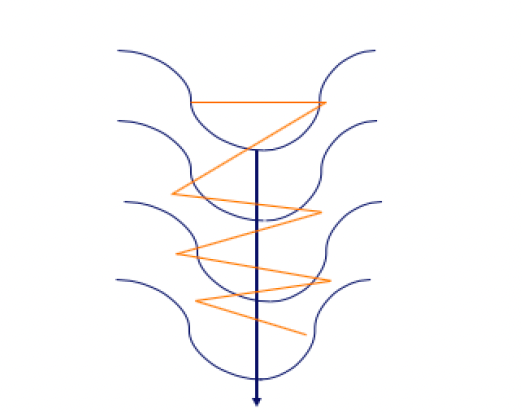
Optimization Paths: Gradient Descent vs. Ideal Trajectory to Global Optimum
To visualise the difference between the SGD and SGD Momentum, let’s look at the following figure:
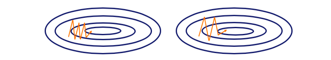
Comparing Gradient Descent Paths in Different Optimization Landscapes
On the left hand-side is the SGD method without Momentum. On the right hand-side is the SGD with Momentum. The orange pattern represents the path of the gradient in a search of the global minimum. As you can see, in the left figure we have more of these occiliations compared to the right one, and that's the impact of Momentum, where we accelerate the training and the algorithm then make less of this movements.
The idea behind the momentum is that the model parameters are learned by using the directions and values of previous parameter adjustments. Also, the adjustment values are calculated in such a way that more recent adjustments are weighted heavier (they get larger weights) compared to the very early adjustments (they get smaller weights).
Example of SGD with Momentum in Python
Let's see what this looks like in code:
def initialize_velocity(parameters):
    """
    Initializes the velocity as a python dictionary with:
                - keys: "dW1", "db1", ..., "dWL", "dbL"
                - values: numpy arrays of zeros of the same shape as the corresponding gradients/parameters.
    """
    L = len(parameters) // 2 # number of layers in the neural networks
    v = {}

    for l in range(L):
        v["dW" + str(l+1)] = np.zeros_like(parameters["W" + str(l+1)])
        v["db" + str(l+1)] = np.zeros_like(parameters["b" + str(l+1)])

    return v

def update_parameters_with_momentum(parameters, grads, v, beta, learning_rate):
    """
    Update parameters using Momentum

    Arguments:
    parameters -- python dictionary containing your parameters
    grads -- python dictionary containing your gradients for each parameters
    v -- python dictionary containing the current velocity
    beta -- the momentum hyperparameter, scalar
    learning_rate -- the learning rate, scalar

    Returns:
    parameters -- python dictionary containing your updated parameters
    v -- python dictionary containing your updated velocities
    """

    L = len(parameters) // 2 # number of layers in the neural networks

    # Momentum update for each parameter
    for l in range(L):
        # compute velocities
        v["dW" + str(l+1)] = beta * v["dW" + str(l+1)] + (1 - beta) * grads["dW" + str(l+1)]
        v["db" + str(l+1)] = beta * v["db" + str(l+1)] + (1 - beta) * grads["db" + str(l+1)]
        # update parameters
        parameters["W" + str(l+1)] = parameters["W" + str(l+1)] - learning_rate * v["dW" + str(l+1)]
        parameters["b" + str(l+1)] = parameters["b" + str(l+1)] - learning_rate * v["db" + str(l+1)]

    return parameters, v
In this code we have two functions for implementing the momentum-based gradient descent algorithm (SGD with momentum):
initialize_velocity(parameters): This function initializes the velocity for each parameter in the neural network. It takes the current parameters as input and returns a dictionary (v) with keys for gradients ("dW1", "db1", ..., "dWL", "dbL") and initializes the corresponding values as numpy arrays filled with zeros.
update_parameters_with_momentum(parameters, grads, v, beta, learning_rate): This function updates the parameters using Momentum optimization technique. It takes the following arguments:
parameters: dictionary containing current parameters of the neural network.
grads: dictionary containing the gradients of the parameters.
v: dictionary containing the current velocities of the parameters (initialized using the initialize_velocity (function).
beta: momentum hyperparameter, a scalar that controls the influence of past gradients on the updates.
learning_rate: learning rate, a scalar controlling the step size of the parameter updates.
Inside the function, it iterates through the layers of the neural network and performs the following steps for each parameter:
Computes new velocity using the momentum formula.
Updates parameter using new velocity and learning rate.
Finally, it returns the updated parameters and velocities.
RMSProp
Root Mean Square Propagation, commonly called RMSprop, is an optimization method with an adaptive learning rate. It was proposed by Geoff Hinton in his Coursera class.
RMSprop adjusts learning rate for each parameter by dividing the learning rate for a weight by a running average of magnitudes of recent gradients for that weight.
RMSprop can be defined mathematically as follows:
$$v_t = \beta v_{t-1} + (1 - \beta) g_t^2$$
$$\theta_{t+1} = \theta_t - \frac{\eta}{\sqrt{v_t + \epsilon}} \cdot g_t$$
_vt_ is the running average of the squared gradients.
β is the decay rate that controls the moving average (usually set to 0.9).
η is the learning rate.
ϵ is a small scalar used to prevent division by zero (usually around 10^-8).
_gt_ is the gradient at time step t, and _θt_ is parameter vector at time step t.
The algorithm first calculates the running average of the squared gradients (the hessian) for each parameter: v_t at step t.
Then it divides the learning rate eta by the square root of this average velocity (element-wise division if the parameters are vectors or matrices). Then it uses this in the same step to update the parameters.
Example of RMSProp in Python
Here's an example of how it works in Python:
def update_parameters_with_rmsprop(parameters, grads, s, learning_rate, beta, epsilon):
    """
    Update parameters using RMSprop.

    Arguments:
    parameters -- python dictionary containing your parameters
                    (e.g., {"W1": W1, "b1": b1, "W2": W2, "b2": b2})
    grads -- python dictionary containing your gradients to update each parameters
                    (e.g., {"dW1": dW1, "db1": db1, "dW2": dW2, "db2": db2})
    s -- python dictionary containing the running average of the squared gradients
                    (e.g., {"dW1": s_dW1, "db1": s_db1, "dW2": s_dW2, "db2": s_db2})
    learning_rate -- the learning rate, scalar.
    beta -- the momentum hyperparameter, scalar.
    epsilon -- small number to avoid division by zero, scalar.

    Returns:
    parameters -- python dictionary containing your updated parameters
    s -- python dictionary containing the updated running average of the squared gradients
    """

    L = len(parameters) // 2 # number of layers in the neural networks

    # Update rule for each parameter
    for l in range(L):
        # Compute moving average of the squared gradients
        s["dW" + str(l+1)] = beta * s["dW" + str(l+1)] + (1 - beta) * np.square(grads["dW" + str(l+1)])
        s["db" + str(l+1)] = beta * s["db" + str(l+1)] + (1 - beta) * np.square(grads["db" + str(l+1)])

        # Update parameters
        parameters["W" + str(l+1)] -= learning_rate * grads["dW" + str(l+1)] / (np.sqrt(s["dW" + str(l+1)]) + epsilon)
        parameters["b" + str(l+1)] -= learning_rate * grads["db" + str(l+1)] / (np.sqrt(s["db" + str(l+1)]) + epsilon)

    return parameters, s
This code defines a function for updating neural network parameters using the RMSprop optimization technique. Here's a summary of the function:
- update_parameters_with_rmsprop(parameters, grads, s, learning_rate, beta, epsilon): function updates parameters of a neural network using RMSprop.
It takes the following arguments:
parameters: dictionary containing current parameters of the neural network.
grads: dictionary containing gradients of the parameters.
s: dictionary containing running average of squared gradients for each parameter.
learning_rate: learning rate, a scalar.
beta: momentum hyperparameter, a scalar.
epsilon: A small number added to prevent division by zero, a scalar.
Inside this function, the code iterates through the layers of the neural network and performs the following steps for each parameter:
Computes the moving average of the squared gradients for both weights (W) and biases (b) using the RMSprop formula.
Updates the parameters using the computed moving averages and the learning rate, with an additional epsilon term in the denominator to avoid division by zero.
Finally, the code returns updated parameters and updated running average of the squared gradients (s).
RMSprop is an optimization technique that adapts the learning rate for each parameter based on the history of squared gradients. It helps stabilize and accelerate training, particularly when dealing with sparse or noisy gradients.
Adam Optimizer
Another popular technique for enhancing the SGD optimization procedure is the Adaptive Moment Estimation (Adam) introduced by Kingma and Ba (2015). Adam basically combines SGD momentum with RMSProp.
The main difference compared to the SGD with momentum, which uses a single learning rate for all parameter updates, is that the Adam algorithm defines different learning rates for different parameters.
The algorithm calculates the individual adaptive learning rates for each parameter based on the estimates of the first two moments of the gradients (first and the second order derivative of the Loss function).
So, each parameter has a unique learning rate, which is being updated using the exponential decaying average of the first moments (the mean) and second moments (the variance) of the gradients.
Basically, Adam, computes individual adaptive learning rates for different parameters from estimates of 1st and 2nd moments of gradients.
The update rules for the Adam optimizer can be expressed as follows:
Calculate running averages of both the gradients and squared gradients
Adjust these running averages for a bias factor
Use these running averages to update the learning rate for each parameter individually
Mathematically, these steps are represented as follows:
$$m_t = \beta_1 m_{t-1} + (1 - \beta_1) g_t$$
$$v_t = \beta_2 v_{t-1} + (1 - \beta_2) g_t^2$$
$$\hat{m}_t = \frac{m_t}{1 - \beta_1^t}$$
$$\hat{v}t = \frac{v_t}{1 - \beta_2^t}$$
$$\theta{t+1} = \theta_t - \alpha \cdot \frac{\hat{m}_t}{\sqrt{\hat{v}_t} + \epsilon}$$
_mt_ and vt are estimates of the first moment (the mean) and the second moment (the uncentered variance) of the gradients, respectively.
m_hat and v_hat are bias-corrected versions of these estimates.
_β_1 and _β_2 are the exponential decay rates for these moment estimates (usually set to 0.9 & 0.999, respectively).
α is the learning rate.
ϵ is a small scalar used to prevent division by zero (usually around 10^(–8)).
Example of Adam in Python
Here's an example of using Adam in Python:
def initialize_adam(parameters) :
    """
    Initializes v and s as two python dictionaries with:
                - keys: "dW1", "db1", ..., "dWL", "dbL"
                - values: numpy arrays of zeros of the same shape as the corresponding gradients/parameters.
    """

    L = len(parameters) // 2 # number of layers in the neural networks
    v = {}
    s = {}

    for l in range(L):
        v["dW" + str(l+1)] = np.zeros_like(parameters["W" + str(l+1)])
        v["db" + str(l+1)] = np.zeros_like(parameters["b" + str(l+1)])
        s["dW" + str(l+1)] = np.zeros_like(parameters["W" + str(l+1)])
        s["db" + str(l+1)] = np.zeros_like(parameters["b" + str(l+1)])

    return v, s

def update_parameters_with_adam(parameters, grads, v, s, t, learning_rate=0.01,
                                beta1=0.9, beta2=0.999, epsilon=1e-8):
    """
    Update parameters using Adam

    Arguments:
    parameters -- python dictionary containing your parameters:
                    parameters['W' + str(l)] = Wl
                    parameters['b' + str(l)] = bl
    grads -- python dictionary containing your gradients for each parameters:
                    grads['dW' + str(l)] = dWl
                    grads['db' + str(l)] = dbl
    v -- Adam variable, moving average of the first gradient, python dictionary
    s -- Adam variable, moving average of the squared gradient, python dictionary
    learning_rate -- the learning rate, scalar.
    beta1 -- Exponential decay hyperparameter for the first moment estimates
    beta2 -- Exponential decay hyperparameter for the second moment estimates
    epsilon -- hyperparameter preventing division by zero in Adam updates

    Returns:
    parameters -- python dictionary containing your updated parameters
    v -- Adam variable, moving average of the first gradient, python dictionary
    s -- Adam variable, moving average of the squared gradient, python dictionary
    """

    L = len(parameters) // 2                 # number of layers in the neural networks
    v_corrected = {}                         # Initializing first moment estimate, python dictionary
    s_corrected = {}                         # Initializing second moment estimate, python dictionary

    # Perform Adam update on all parameters
    for l in range(L):
        # Moving average of the gradients.
        v["dW" + str(l+1)] = beta1 * v["dW" + str(l+1)] + (1 - beta1) * grads["dW
In this code we implement Adam algorithm, consisting of two functions:
initialize_adam(parameters): This function initializes the Adam optimizer variables
vandsas two Python dictionaries. It takes the current parameters as input and returnsvands, both of which are dictionaries with keys for gradients ("dW1", "db1", ..., "dWL", "dbL"). The values are numpy arrays filled with zeros and have the same shape as the corresponding gradients/parameters.update_parameters_with_adam(parameters, grads, v, s, t, learning_rate=0.01, beta1=0.9, beta2=0.999, epsilon=1e-8): This function updates the parameters of a neural network using the Adam optimization technique. It takes the following arguments:
parameters: A dictionary containing the current parameters of the neural network.
grads: A dictionary containing the gradients of the parameters.
v: A dictionary representing the moving average of the first gradient moments.
s: A dictionary representing the moving average of the squared gradient moments.
t: A scalar representing the current time step (used for bias correction).
learning_rate: The learning rate, a scalar.
beta1: The exponential decay hyperparameter for the first moment estimates.
beta2: The exponential decay hyperparameter for the second moment estimates.
epsilon: A small number added to prevent division by zero in Adam updates.
Inside this function, code iterates through layers of the neural network and performs Adam updates for each parameter. This includes computing moving averages of gradients and squared gradients, and using these values to update the parameters. It also performs bias correction to adjust the moving averages.
Finally, code returns the updated parameters, v (first moment estimates), and s (second moment estimates).
AdamW
AdamW (the 'W' stands for 'Weight Decay') is a optimization algorithm which modifies the way weight decay is integrated into the original Adam algorithm. This seemingly small change has significant implications for the training process, particularly in how it manages regularization to prevent overfitting.
This step has a crucial impact in making deep learning model more generalizable, for building models that generalize well to new, unseen data.
In traditional optimizers like SGD, the weight decay directly regularizes the model's weight parameters. But, in Adam, this process is somewhat conflated with the optimizer's adaptive learning rates.
AdamW decouples weight decay from the learning rates, reinstating the direct regularization effect seen in SGD. This results in more effective regularization and, often, better performance in training deep neural networks.
If you want to see the actual mathematical representation where I am comparing Adam and AdamW, you can check out this Tutorial on YouTube.
By choosing AdamW, you can enjoy the benefits of adaptive learning rates while maintaining a more robust regularization mechanism.
This optimization algorithm has quickly gained popularity in the machine learning community, particularly among those working on large-scale models and complex datasets where every bit of optimization efficiency counts.
AdamW in Python
import numpy as np

def initialize_adamw(parameters):
    """
    Initializes v, s, and w as three python dictionaries with:
                - keys: "dW1", "db1", ..., "dWL", "dbL"
                - values: numpy arrays of zeros of the same shape as the corresponding gradients/parameters.
    """

    L = len(parameters) // 2  # number of layers in the neural network
    v = {}
    s = {}
    w = {}

    for l in range(L):
        v["dW" + str(l+1)] = np.zeros_like(parameters["W" + str(l+1)])
        v["db" + str(l+1)] = np.zeros_like(parameters["b" + str(l+1)])
        s["dW" + str(l+1)] = np.zeros_like(parameters["W" + str(l+1)])
        s["db" + str(l+1)] = np.zeros_like(parameters["b" + str(l+1)])
        w["W" + str(l+1)] = np.copy(parameters["W" + str(l+1)])

    return v, s, w

def update_parameters_with_adamw(parameters, grads, v, s, w, t, learning_rate=0.01,
                                beta1=0.9, beta2=0.999, epsilon=1e-8, weight_decay=0.01):
    """
    Update parameters using AdamW (Adam with weight decay)

    Arguments:
    parameters -- python dictionary containing your parameters:
                    parameters['W' + str(l)] = Wl
                    parameters['b' + str(l)] = bl
    grads -- python dictionary containing your gradients for each parameter:
                    grads['dW' + str(l)] = dWl
                    grads['db' + str(l)] = dbl
    v -- Adam variable, moving average of the first gradient, python dictionary
    s -- Adam variable, moving average of the squared gradient, python dictionary
    w -- Weight parameters for weight decay, python dictionary
    t -- Current time step (used for bias correction), scalar
    learning_rate -- The learning rate, scalar
    beta1 -- Exponential decay hyperparameter for the first moment estimates
    beta2 -- Exponential decay hyperparameter for the second moment estimates
    epsilon -- Hyperparameter preventing division by zero in Adam updates
    weight_decay -- Weight decay hyperparameter, scalar

    Returns:
    parameters -- python dictionary containing your updated parameters
    v -- Adam variable, moving average of the first gradient, python dictionary
    s -- Adam variable, moving average of the squared gradient, python dictionary
    """

    L = len(parameters) // 2  # number of layers in the neural network
    v_corrected = {}          # Initializing first moment estimate, python dictionary
    s_corrected = {}          # Initializing second moment estimate, python dictionary

    # Perform AdamW update on all parameters
    for l in range(L):
        # Moving average of the gradients
        v["dW" + str(l+1)] = beta1 * v["dW" + str(l+1)] + (1 - beta1) * grads["dW" + str(l+1)]
        v["db" + str(l+1)] = beta1 * v["db" + str(l+1)] + (1 - beta1) * grads["db" + str(l+1)]

        # Moving average of the squared gradients
        s["dW" + str(l+1)] = beta2 * s["dW" + str(l+1)] + (1 - beta2) * np.square(grads["dW" + str(l+1)])
        s["db" + str(l+1)] = beta2 * s["db" + str(l+1)] + (1 - beta2) * np.square(grads["db" + str(l+1)])

        # Bias correction for moving averages
        v_corrected["dW" + str(l+1)] = v["dW" + str(l+1)] / (1 - np.power(beta1, t))
        v_corrected["db" + str(l+1)] = v["db" + str(l+1)] / (1 - np.power(beta1, t))
        s_corrected["dW" + str(l+1)] = s["dW" + str(l+1)] / (1 - np.power(beta2, t))
        s_corrected["db" + str(l+1)] = s["db" + str(l+1)] / (1 - np.power(beta2, t))

        # Update parameters with weight decay
        parameters["W" + str(l+1)] -= learning_rate * (v_corrected["dW" + str(l+1)] / (np.sqrt(s_corrected["dW" + str(l+1)]) + epsilon) + weight_decay * w["W" + str(l+1)])
        parameters["b" + str(l+1)] -= learning_rate * (v_corrected["db" + str(l+1)] / (np.sqrt(s_corrected["db" + str(l+1)]) + epsilon) + weight_decay * w["W" + str(l+1)])

    return parameters, v, s
In this code we implement AdamW optimization algorithm, which is an extension of the Adam optimizer with added weight decay regularization. Let's go through each part of the code:
- initialize_adamw(parameters): This function initializes AdamW optimizer variables. It takes all the current parameters of a neural network as input and returns three dictionaries:
v,s, andw.
Here's what each of these dictionaries represents:
v: A dictionary for the moving average of the first gradient moments. It has keys like "dW1", "db1", ..., "dWL", "dbL", and the values are initialized as numpy arrays filled with zeros of the same shape as the corresponding gradients/parameters.
s: A dictionary for the moving average of the squared gradient moments, similar to
v.w: A dictionary for weight parameters used for weight decay. It is initialized with a copy of the current weight parameters.
update_parameters_with_adamw(parameters, grads, v, s, w, t, learning_rate=0.01, beta1=0.9, beta2=0.999, epsilon=1e-8, weight_decay=0.01): This function performs AdamW as we saw in the equations, to update on the neural network parameters. It takes several arguments:
parameters: A dictionary containing the current parameters of the neural network.
grads: A dictionary containing the gradients of the parameters, calculated during backpropagation.
v: dictionary representing the moving average of the first gradient moments.
s: dictionary representing the moving average of the squared gradient moments.
w: dictionary containing weight parameters for weight decay.
t: scalar representing the current time step (used for bias correction).
learning_rate: The learning rate, a scalar.
beta1: exponential decay hyperparameter for the first moment estimates (typically close to 1).
beta2: exponential decay hyperparameter for the second moment estimates (typically close to 1).
epsilon: small number added to prevent division by zero in Adam updates.
weight_decay: weight decay hyperparameter, which controls the strength of L2 regularization.
Inside the function, the following steps are performed for each parameter:
Update
vandsusing the gradients, similar to the standard Adam update.Perform bias correction on
vandsto account for the fact that they are initialized with zeros and may be biased towards zero.Update parameters with weight decay regularization. Weight decay encourages smaller parameter values by subtracting a fraction of the current weight from the update.
Return the updated parameters,
v, ands.
Chapter 5: Regularization and Generalization
In this chapter, we'll dive into some important concepts in Deep Learning, like:
Overfitting & underfitting in neural networks
Regularization techniques: Dropout, L1/L2 regularization, batch normalization
Data augmentation & its role in improving model robustness
Let's get started.
The Dropout Regularization Technique
Dropout is one of the most popular regularization techniques used to prevent overfitting in neural networks. The way the algorithm works is that it randomly “drops out” (that is, it sets to zero) a number of output features of the layer during training.
During the training process, after calculating the activations, the algorithm randomly sets fraction p (the dropout rate) of the activations to zero. These features are then not being used during the training process in that pass. This dropout rate p is a hyperparameter typically set between 0.2 and 0.5. Note that this drop-out rate is only used during training.
For each layer l, for each training example i, and for each neuron/unit j, the dropout can be mathematically represented as follows:
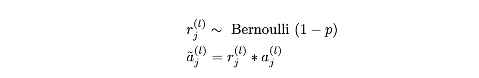
Where:
rj(l) is a random variable that follows Bernoulli distribution, where the probability of not being dropped out (success: 1) is 1−_p_.
aj(l) is the activation of neuron j in layer l.
a~j(l) is the activation of neuron j after applying dropout.
During backpropagation in the training process, the gradients are only passed through the neurons that were not dropped out (when there was a success in Bernoulli trial). Remember that this drop-out rate is only used during training.
Testing Adjustment: During testing process, the dropout is not applied. Instead, the activations are scaled down by a factor of p to account for the effect of dropout during training process. This is necessary because during training, on average, each unit is only active with probability 1−_p_.
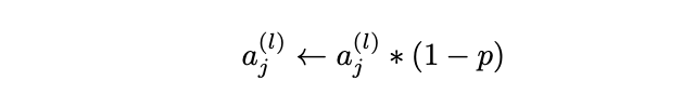
This ensures that the expected sum of the activations is the same during training and test time.
Dropout effectively creates a “thinned” network with a different architecture for each training step. Because the network architecture is different for each training sample as we randomly turn off some of the neurons, this can be seen as of training a collection of networks with shared weights.
During testing, you get the benefit of averaging the effects of these different networks, which tends to reduce overfitting. This is because it introduces beat bias, but more importantly, it significantly reduces variance when the model is used for prediction. Here’s why:
Introducing Bias
By dropping out different subsets of neurons with rate p, the network is then forced to learn more robust features that are useful in conjunction with many different random subsets of the other neurons.
This adjustment might lead to a slightly higher bias during training because the network is less likely to learn patterns that are highly specific to the training data (which can be thought of as noise).
Decreasing Variance
Dropout reduces the variance by preventing the network from becoming too fitted to the training data. It reduces the risk that the network relies on any one feature, thereby ensuring that the model generalizes better to unseen data.
This is common to ensemble methods in machine learning like Boosting, Random Forest, where averaging of different models’ predictions leads to a reduction in variance.
Ridge Regularization (L2 Regularization)
Lasso and Ridge regularization are techniques originally developed for linear models, but they can also be applied to deep learning. In deep learning, these regularization methods work similarly by adding a penalty to the loss function, but they have to be adapted to the context of neural networks. Here’s how they function in deep learning:
Ridge regularization, also referred as L2 regularization adds a penalty equal to the square of the magnitude of coefficients as shown below. This L_L2 shows the penalization term that is added to the loss function of the nerual network For neural networks, this means the penalty is the sum of the squares of all the weights in the network.
$$L2 = \lambda \sum w_i^2$$
where lambda is the penalization parameter, w_i are the weights of the neural network.
The effect of this is that it encourages the weights to be small but doesn’t force them to zero.
This is useful for deep learning models where we don’t necessarily want to perform feature selection (reduce dimension of the model) but just want to prevent overfitting by discouraging overly complex models that memorizes the training data and not generalizable.
This regularization term is controlled by a hyperparameter, often denoted by the Greek letter λ, which determines the strength of this penalty. As λ increases, penalty for larger weights increases, and the model is pushing towards smaller weights.
Lasso Regularization (L1 Regularization)
Lasso stands for Least Absolute Shrinkage and Selection Operator Regularization, also known as L1 regularization based on L1 norm.
L1 regularization adds a penalty equal to the absolute value of the magnitude of coefficients (the sum of them). The formula below shows the L_L1 penalization term added to the loss function of the neural network. The notions, are the same as in case of the Ridge Regularization. This translates to neural networks in deep learning as the sum of the absolute values of all the weights.
$$L1 = \lambda \sum |w_i|$$
L1 regularization drives some weights to be exactly zero, thus achieving sparse models. In deep learning, this can lead to sparsity within the weights, effectively performing a form of feature selection by allowing the model to ignore certain inputs.
Similar to L2 regularization, the strength of L1 regularization is controlled by a hyperparameter, which when increased, can lead to more weights being set to zero.
L1 and L2 regularization can be used individually or combined in what’s known as Elastic Net regularization as a way to regularize the network.
Using these regularization techniques can improve the generalization of deep learning models. But it’s also important to consider other techniques more common in deep learning, such as dropout and batch normalization – or use all of them together (which can sometimes be more effective in preventing overfitting in large and deep neural networks).
If you want to learn more details about L1/L2 regularisation make sure to check this video and this tutorial to see how these regularization techniques penalize the weights in neural network which are part of my free Deep Learning Interview Preparation Course.
Batch Normalization
Batch Normalization is another important technique used in Deep Learning that, while not a regularization method in the traditional sense, has an indirect regularization effect.
This technique normalizes the inputs of each layer in such a way that they have a mean output activation of zero, and s standard deviation of one. Basically like Gaussian Distribution – which is the reason why it’s called Normalization, as we are normalizing a batch.
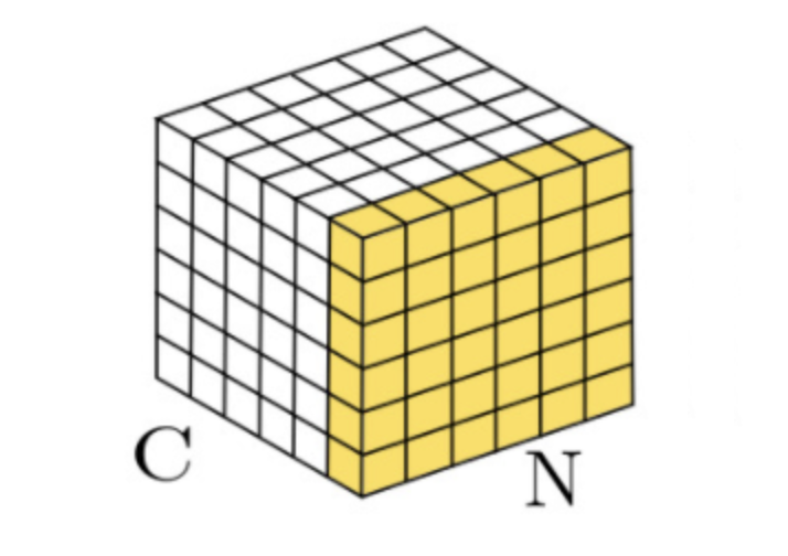
Batch Normalization: Image Source
Figure above, visualizes the idea behind Batch Normalization, which shows that normalization is done for each batch, where all N observations are in 1 batch, and C represents the number of Channels or features in your data. Basically, this figure shows that batch normalization is normalizing the data per 1 feature (across single channel) and for all N observations in 1 batch.
This is achieved by adjusting and scaling the activations during training. Batch normalization allows each layer of a network to learn by itself a little more independently of other layers. Let's see how it works in more detail.
Step 1: Mini-batch Mean & Variance:
Compute the mean of the activations for a mini-batch using the following equation:
$$\mu_B = \frac{1}{m} \sum_{i=1}^{m} x_i$$
In this equation,
_μ_beta_ is the mean of the mini-batch
m is the number of training examples in mini-batch, and
_xi_ is the activation of the current layer before batch normalization.
Now, you'll need to compute the variance of the activations for a mini-batch. You can do that using the following equation:
$$\sigma_B^2 = \frac{1}{m} \sum_{i=1}^{m} (x_i - \mu_B)^2$$
Step 2: Normalize activations of the mini-batch
Then the normalization happens:
$$\hat{x}_i = \frac{x_i - \mu_B}{\sqrt{\sigma_B^2 + \epsilon}}$$
In this equation,
x^_i_ is the normalized activation
ϵ is a small constant added for numerical stability (to avoid division by zero).
Step 3: Apply the learnable parameters for scale and shift
$$y_i = \gamma \hat{x}_i + \beta$$
While the primary goal of batch normalization is to stabilize and accelerate deep neural networks’ training process by reducing internal covariate shift, it also has a regularization effect which is the way of reducing overfitting.
By adding some level of noise to the activations (since the mean and variance are estimated from the data), it can make the model less sensitive to the specific weights of neurons, which has a similar effect to dropout as it can prevent overfitting.
Batch normalization can be particularly beneficial in deep neural networks, where it can enable the use of higher learning rates, make the network less sensitive to the initialization, and can reduce need for other regularization techniques such as dropout.
In practice, batch normalization is applied before the activation function of a layer, and it requires maintaining a running average of the mean and variance to be used during inference for the normalization process.
Chapter 6: Vanishing Gradient Problem
As the gradient of the loss is propagated backward through time and layers, it can shrink towards 0 (becoming very small). This leads to very small updates to the weights.
This makes it hard for neural network to learn long-range dependencies, resulting in potentially no updates in the earlier layers of the network in the parameters as the gradients vanishes (become very small, close to zero).
So, when gradients vanish, early layers in the network train very slowly or not at all, leading to suboptimal performance.
Use appropriate activation functions
One way of solving the vanishing gradient problem is by using an appropriate activation function that doesn't suffer from saturation.
Saturation happens when, for the input value x that is a large positive number or a small negative number, the gradient of the function is close to 0 as the function value is in the neighbourhood of the static extreme values of it. This slows down the parameter update. This phenomenon is called the saturation problem.
The ReLU (Rectified Linear Unit) and Leaky ReLU activation functions do not saturate in the positive direction, unlike the Sigmoid or tanh functions. This can help mitigate the vanishing gradient problem.
Leaky ReLU can help further by allowing a small, non-zero gradient when the unit is not active. This is important for cases when the negative inputs should also be taking into account and potentially getting negative value in the output is acceptable.
You can find more details on this activation function in the section on Activation Functions in Chapter 2.
Use Xavier or He Initialization
Initializing weights carefully is important. A good initialization as such the Xavier initialization can help to prevent gradients from becoming too small early in training.
Xavier initialization, which is also known as Glorot initialization, is a an initialization technique for the weight parameters in a neural network. It is designed to solve the problem of vanishing or exploding gradients in deep neural networks when Sigmoid and tanh activation functions are being used.
It is named after Xavier Glorot who formulated this strategy based on the understanding of the flow of variances through a neural network to maintain the gradients at a reasonable scale and prevent them from becoming too small to vanish or too large to explode.
Here’s the main idea behind Xavier Initialization:
For a given layer, the weights are initialized randomly from a distribution with mean 0 and a specific variance (can also be 1 like in Gaussian distribution) that depends on the number of input neurons and the number of output neurons.
The goal of Xavier Initialization is to have the variance of the outputs of each layer to be equal to the variance of its inputs, and the gradients to have equal variance before and after going through a layer in the backward propagation.
If it's a Uniform Distribution, the weights are usually initialized with values drawn from this calculation:
$$W \sim \text{Uniform}\left(-\sqrt{\frac{6}{n_{\text{in}} + n_{\text{out}}}}, \sqrt{\frac{6}{n_{\text{in}} + n_{\text{out}}}}\right)\$$
$$\text{Var}(W) = \frac{2}{\sqrt{n_{\text{in}} + n_{\text{out}}}}$$
This variance for initializing the weights in Neural Network is typically set to this value above referred by Var(W) - as in Variance of Weights matrix W, where:
_n__in is the number of neurons feeding into the layer
_n__out is the number of neurons the results are fed into (that is, number of neurons in the next layer)
If a Normal Distribution is used instead, then the weights are drawn from this one:
$$W \sim \text{Normal}\left(0, \sqrt{\frac{2}{n_{\text{in}} + n_{\text{out}}}}\right)\$$
$$\text{Var}(W) = \frac{2}{\sqrt{n_{\text{in}} + n_{\text{out}}}}$$
Perform Batch Normalization
Performing batch normalization on the input layer can help maintain a mean output close to 0 and a standard deviation close to 1 like Standard Normal Distribution. This prevents the gradients from becoming too small.
By Normalizing the activations, you directly stabilize the network but indirectly also control the weights change of your network. This means that the gradients stay more constant, and as an indirect result, BatchNorm gradients will not vanish nor explode.
Add Residual Connections (especially to RNNs or LSTMs)
Residual connections offer innovative optimization results for training deep neural networks, especially when it comes to combating the vanishing gradients problem.
This is particularly a problem when dealing with recurrent neural networks (RNNs) or Long Short-Term Memory networks (LSTMs), which are inherently deep due to their sequential nature. Incorporating residual connections into RNNs or LSTMs can significantly improve their learning capabilities.
RNNs and LSTMs are specialized for handling sequences of data, making them ideal for tasks like language modeling and time series analysis. But as the sequence length increases, these networks tend to suffer from the vanishing gradient problem.
To address this, often residual connections are used for RNNs and LSTMs. By adding a shortcut that bypasses one or more layers, a residual connection allows the gradient to flow through the network more directly. In the context of RNNs and LSTMs. This means connecting the output of one timestep not only to the next timestep but also to one or several subsequent timesteps.
How to Implement Residual Connections in RNNs and LSTMs
The implementation strategy for residual connections in RNNs and LSTMs is straightforward. For each timestep, we modify the network such that the output is not only a function of the current input and the previous hidden state, but so that it also includes the input directly.
This process can be described as follows where we add x to output F(x). You can also see the direct path for the gradient to flow into the network and the mathematical derivation based on this process of adding input to output:
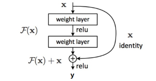
Gradient Clipping (Image Source: LunarTech.ai)
$$y = x + F(x)\$$
$$\frac{\partial E}{\partial x} = \frac{\partial E}{\partial y} \cdot \frac{\partial y}{\partial x}\$$
$$\frac{\partial E}{\partial x} = \frac{\partial E}{\partial y} \cdot (1 + F'(x))\$$
$$\frac{\partial E}{\partial x} = \frac{\partial E}{\partial y} \cdot F'(x)$$
Here you can see the mathematics behind Residual Connections and how the gradient gets the short-cut. When we add x on F(x) to get y, instead of just y=F(x), you can see that when we take the derivative of some function E (let's say our loss function) with regard to x. Then we use the chain rule from differential mathematics.
After these transformations, you can see that we end up having sum of two values:
Gradient of loss function with regard to y
Gradient of loss function with regard to y multiplied by partial derivative of F(x) with regard to x
So, you can see here, that in case when residual connection is done, and we add extra x the plain y = F(x) , then this end up adding extra Gradient of loss function with regard to y without any other multiplication factor to be added to the final gradient.
For intuitive and detailed explanation, check out this tutorial-interview answer on Residual Connections.
Direct Gradient Flow: By providing a shortcut for the gradient to flow, it is less likely to vanish as it is propagated back through time. This ensures that even the earliest layers in the sequence can be effectively trained.
Learning Identity Mappings: If the optimal function for a timestep is to copy its input to the output, the network can learn this identity mapping more easily with residual connections. The network can thus focus on fine-tuning deviations from the identity rather than learning it from scratch.
Facilitating Deeper Architectures: With the integration of residual connections, it becomes feasible to construct deeper RNNs or LSTMs. This depth allows the network to learn more complex patterns and relationships within the data.
Chapter 7: Combatting Exploding Gradients
Exploding gradients is the opposite problem of Vansihing Gradients. Exploding Gradients occur when in the training of deep learning models, particularly those involving neural networks during the backpropagation phase, the gradients become too large and they basically explode.
But in deep networks with many layers, these gradients can accumulate and grow exponentially large through each layer. This exponential increase is due to the repetitive multiplication of gradients through the network's depth, especially when the gradients are too large in their magnitude.
This hinders the learning process and makes the neural network less effective in learning the important information in the layers.
Let's look at how we can solve this problem.
Gradient Clipping
One way of solving the exploding gradients problem is by using Gradient Clipping. Gradient clipping is a practical technique that is used to prevent gradients from exploding during the training of neural networks.
When the computed gradients are too large, gradient clipping scales them back to a predefined threshold. This ensures stable and consistent updates to the model's parameters.
This process involves:
Step 1: Calculating gradient (g): Obtain the gradient of the loss function with respect to the model's parameters.
Step 2: Scaling gradient: If the norm of this gradient ∥_g_∥ is larger than a specified threshold c, we scale down gradient g to have the norm c, maintaining its direction. This is done by setting g to c_⋅_g/∥_g_∥
Step 3: Update parameters: We use the clipped gradient for a controlled and more moderate update.
Gradient clipping ensures that the model's learning process does not derail due to these large updates as a result of exploding gradients, which can happen in the presence of steep slopes in the loss landscape when optimization should happen after backpropagation.
By keeping these updates of the weight and bias parameters within a 'safe' size, this method helps in navigating the loss landscape more smoothly, contributing to better training convergence. The threshold c_c_ is a hyperparameter that requires tuning to balance between adequate learning speed and stability.
Chapter 8: Sequence Modeling with RNNs & LSTMs
In this chapter, you'll learn about one of the most popular type of Neural Network models, Recurrent Neural Networks (RNNs).
Sequence modeling is a cornerstone of deep learning for sequential data such as time-series, speech, and text. We’ll look into the mechanics of RNNs, their inherent limits, and the evolution of advanced architectures such as Long Short-Term Memory (LSTM).
Recurrent Neural Networks (RNN) Architecture
RNNs stand out for their unique ability to form a directed graph along a sequence, allowing them to exhibit temporal dynamic behavior. Unlike feedforward, in usual neural networks, RNNs can use their internal state (memory) to process sequences of inputs.
At the core of RNN is the concept of a cell, which is the repeating unit that forms the base of the RNN’s ability to maintain a memory across input sequences (the tine and sequence element). At high level, RNN can be visualized as follows:
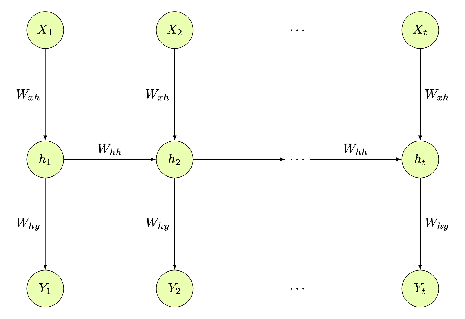
RNN architecture (Image Source: LunarTech.ai)
This visualization makes understanding this more complex architecture easier. As you can see in the image, the hidden layer used on a specific observation of a data set is not only used to generate an output for that observation (output y using h_t), but it is also used to train the hidden layer of the next observation (h_t is used with x_(t+1) to get the h_(t+1)).
Unlike basic Neural Networks that have a single input, multiple independent hidden layers, and then single output Y, RNNs have a different architecture.
Besides having a different structure for input and output (that is, multiple inputs and outputs), the most important thing to notice here is that in an RNN's hidden layers, the hidden states are interconnected.
This “dependent” property of one observation helping to predict the next observation is why recurrent neural networks are so handy when it comes to problems with time or sequence elements (such as time series analysis problems or next-word prediction problems form NLP).
Recurrent Neural Network Pseudocode
For the start, let’s look for instance at the first time step. The hidden state at time step 1 is calculated as follows:
$$h_1 = f(W_{xh} \cdot X_1 + W_{hh} \cdot h_0 + b_h)$$
where:
f is an activation function (like ReLU or Tanh)
W_xh is the input-to-hidden weight matrix
W_hh is the hidden-to-hidden weight matrix
h_0 is the initial hidden state (previous)
b_h is the hidden layer bias
W_hh is often referred to as the recurrent weight matrix. This is the matrix that defines how much each of those previous hidden states will contribute to the computation of the present hidden state.
Then the output in this first time-step is the following:
$$Y_1 = W_{hy} \cdot h_1 + b_y$$
where:
_W_hy_ is the weight matrix from hidden to output layer
_b_y_ is the bias for the output layer
The RNN algorithm for all time-steps 1 till T can be described with the following pseudocode:
Algorithm 1 Recurrent Neural Network Time Steps
1: for each time step t = 1 to T do
2:     Input: Xt
3:     Initialize: h0 to a vector of zeros
4:     Parameters:
5:         Wxh: Weight matrix from input to hidden layer
6:         Whh: Recurrent weight matrix for hidden layer
7:         Why: Weight matrix from hidden to output layer
8:         bh: Bias for hidden layer
9:         by: Bias for output layer
10:     Activation function: f (e.g., tanh, ReLU)
11:     Hidden State Update:
12:         ht = f(Wxh . Xt + Whh . ht−1 + bh)
13:     Output:
14:         Yt = Why . ht + by
15: end for
Limitations of Recurrent Neural Networks
Now let’s discuss the limitations of RNNs and why LSTMs came into play as well as later on the Transformers! Following are the limitations of the Recurrent Neural Network:
Vanishing Gradient Problem
Exploding Gradient Problem
Serial Computation
Difficulty Handling Long Sequences
Limited Contextual Information
Since we've already discussed the Vanishing and Exploding Gradient problems and how to solve them, we will move on to the remaining limitations of RNN before discussing variations of RNNs that addresses these challenges.
But first, just to note: especially in case of RNNs, Vanishing Gradient can result in the early layers of the network learning very slowly, if at all, which makes RNNs poorly suited to learning long-range dependencies within a sequence. And in the case ofExploding Gradients, they can lead to large updates to network parameters and consequently to an unstable Recurrent Neural Network.
Serial Computation Limitation
The sequential nature of RNNs doesn’t allow for parallelization during training because the computation of the next step depends on the previous step. This can result in much slower training processes compared to neural networks that do allow full parallelization.
Difficulty Handling Long Sequences
RNNs can have difficulty when dealing with long sequences because information from early in the sequence can be lost by the time it reaches the end in case Vanishing Gradient is an issue.
Limited Contextual Information Limitation
This is one of the most important limitations that RNN has that motivated the invention of Transformers. Standard RNNs do not have a mechanism to selectively remember or forget information, which can be a limitation when processing sequences where only certain parts are relevant for the prediction.
Long Short-Term Memory (LSTM) Architecture
Long Short-Term Memory Networks or LSTMs are a special kind of RNN designed to mitigate most of the limitations of traditional RNNs. They incorporate mechanisms that we call Cells that allow the network to regulate the information that flows through it.
These gates are:
Forget Gate: Gate that determines what information should be discarded from the cell state
Input Gate: Gate that updates the cell state with new information
Output Gate: Gate that determines what next hidden state should be
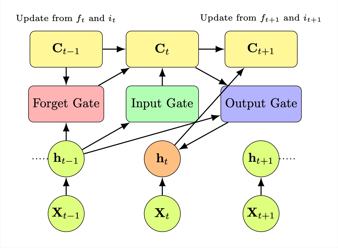
LSTM Architecture (Image Source: LunarTech.ai)
This diagram represents the architecture of an LSTM (Long Short-Term Memory) network, visualizing the flow of data through its components at different time steps, let's dive deeper into each of this sates and the process behind them:
Cell States: At the top row, we have rectangles in yellow labeled C_(t−1), C(t)_, … C(t+1)_. These represent the cell states of LSTM at consecutive time steps.
These cell states are a key component of the LSTM as they carry relevant information throughout processing of the sequence. They hold the information of what information to use, what to forget and what to output.
Arrows indicate the flow and transformations of the cell state from one time step to the next one.
Gates: In the middle you can see the 3 gates, coloured blocks representing the LSTM’s gates:
Forget Gate (Pink): Determines which parts of cell state C(t−1)_ needs to be forgotten and which need to be remembered, to produce the subsequent cell state C(t)_.
Input Gate (Green): Decides which values will be updated in the cell state based on the input at the current time step.
Output Gate (Purple): Determines what part of the cell state will be used to generate the output hidden state _h_t_.
These 3 gates control the flow of information and their amount, with lines connecting the previous hidden state h(t−1) _and the cell state to each of these gates, illustrating how each of them contribute to the current state.
Difference between Cell and Gates: Note, that cells and gates are different concepts, where as you can see from the diagram cell is at higher leven than the gates, and for each time step there is single cell state but 3 gates. Cell state is basically using 3 gates to regulate the flow of information. It's like function that uses 3 input values to generate output to put it simply.
Common to the RNN original architecture, the hidden state at each time step is influenced by the previous hidden state and current input, and also the internal gates’ operations common for LSTMs.
These gates within LSTM allow it to learn which information to keep or discard over time, making it possible to capture long-term dependencies in the data.
How LSTMs address RNN limitations
Solving Vanishing and Exploding Gradients: LSTMs are designed to have a more constant weight changes which means that the gradients are more constant. This allows them to learn over many time steps, thereby solving the vanishing/exploding gradients through their gating mechanism and by maintaining a separate cell state.
Long-range Dependencies: By learning what to store in and what to delete/forget from the cell state, LSTMs can maintain long-range dependencies or relationships in the data. This makes them more effective for tasks involving long sequences such as those in language models.
Selective Memory: LSTMs can learn to keep only relevant information to make predictions by using the, forget gate. Forgetting non-relevant data, which makes them better at modeling complex sequences where the relevance of the information varies with time helps to do exactly this.
Limitations of LSTMs
While LSTMs represent a significant improvement over the original RNNs, they still have some major disadvantages, such as being more computationally intensive due to their complex architecture. LSTM’s have a higher number of parameters, which can lead to longer training times and require more data to generalize effectively.
Also, similar to RNNs, LSTMs also process data sequentially, which means they cannot be fully parallelized.
So, parallelization and longer training time due to higher number of parameters remain two major disadvantages for RNNs and LSTMs.
Chapter 9: Deep Learning Interview Preparation
As we reach the culmination of this comprehensive handbook, it’s time to focus on translating your newfound knowledge into real-world success.
Whether you're aiming for getting into AI industry or eyeing a coveted position for AI Researcher or AI Engineer at FAANG companies, the final hurdle is often the most challenging yet rewarding: the job interview.
You will need to know details and be able to answer tricky questions that go beyond the surface level theory information.
You'll need to know about:
Convolutional Neural Networks (pooling, padding, kernels)
Recurrent Neural Networks (RNN), LSTMs, GRUs
Batch/Layer Normalization
Generative Adverserial Networks (GANs)
AutoEncoders (Encoder-Decoder Architectures)
Variational AutoEncoders (KL Divergence, ELBO)
Embeddings
Multi-Head Attention Mechanism
Transformers
And those are just few topics that you can expect for your more advanced/FAANG interviews. Check out the full list of 100 Questions from this curriculum of here.
Understanding the importance of this critical step, I'm excited to introduce my specially designed Deep Learning Interview Course sponsored by LunarTech that's available on LunarTech.ai and Udemy. This course is meticulously tailored to ensure you are not just interview-ready but poised to excel in the highly competitive AI job market.
Here's what the course covers:
Part 1 – The Essentials (Free 4-Hour Course): I believe in empowering every Data Science AI enthusiast. So I'm offering the first part of my interview course absolutely free. This section includes first set of 50 interview questions that cover the breadth of deep learning fundamentals.
Complete Course - [Full Deep Learning Interview Prep Course - 100 Q&A 7.5 hours ]: For those who are determined to leave no stone unturned, our full course on LunarTech.ai is the ultimate preparation tool for easy but also complex Deep Learning interviews. Expanding to 100 in-depth interview questions, this comprehensive course delves into the nuances of deep learning, ensuring that you stand out in even the most demanding interviews, including companies like FAANG.
It's your opportunity to go beyond being a candidate – to becoming a standout in the field of AI.
About the Author
I am Tatev Aslanyan, Senior Machine Learning and AI Researcher. I have had the privilege of working in Data Science across numerous countries, including the US, UK, Canada, and the Netherlands. I am Co-founder of LunarTech where make Data Science and AI more accessible to everyone!
With an MSc and BSc in Econometrics under my belt, my journey in Machine and AI has been nothing short of incredible. Drawing from my technical studies during my Bachelors & Masters, along with over 5 years of hands-on experience in the Data Science, Machine Learning and AI industry.
Connect with Me and LunarTech

Image Source: [LunarTech](https://lunartech.ai" style="box-sizing: inherit; margin: 0px; padding: 0px; border: 0px; font-style: inherit; font-variant-caps: inherit; font-weight: inherit; font-stretch: inherit; line-height: inherit; font-family: inherit; font-size-adjust: inherit; font-kerning: inherit; font-variant-alternates: inherit; font-variant-ligatures: inherit; font-variant-numeric: inherit; font-variant-east-asian: inherit; font-variant-position: inherit; font-feature-settings: inherit; font-optical-sizing: inherit; font-variation-settings: inherit; font-size: 17.6px; vertical-align: baseline; background-color: transparent; color: var(--gray90); text-decoration: underline; cursor: pointer; word-break: break-word;)
Visit my Personal Website for Free Resources
Subscribe to The Data Science and AI Newsletter
If you want to start a career in Data Science or AI, download my free Data Science and AI Handbook or Fundamentals to Machine Learning Handbook
Best wishes in all your future endeavors!