

If you're planning to become a Machine Learning Engineer, Data Scientist, or you want to refresh your memory before your interviews, this handbook is for you.
In it, we'll cover the key Machine Learning algorithms you'll need to know as a Data Scientist, Machine Learning Engineer, Machine Learning Researcher, and AI Engineer.
Throughout this handbook, I'll include examples for each Machine Learning algorithm with its Python code to help you understand what you're learning.
Whether you're a beginner or have some experience with Machine Learning or AI, this guide is designed to help you understand the fundamentals of Machine Learning algorithms at a high level.
As an experienced machine learning practitioner, I'm excited to share my knowledge and insights with you.
What You'll Learn
2.1 Linear Regression and Ordinary Least Squares (OLS)
2.2 Logistic Regression and MLE
2.3 Linear Discriminant Analysis(LDA)
2.4 Logistic Regression vs LDA
2.5 Naïve Bayes
2.6 Naïve Bayes vs Logistic Regression
2.7 Decision Trees
2.8 Bagging
2.9 Random Forest
2.10 Boosting or Ensamble Techniques (AdaBoost, GBM, XGBoost)
3. Chapter 3: Feature Selection
3.1 Subset Selection
3.2 Regularization (Ridge and Lasso)
3.3 Dimensionality Reduction (PCA)
4. Chapter 4: Resampling Technique
4.1 Cross Validation: (Validation Set, LOOCV, K-Fold CV)
4.2 Optimal k in K-Fold CV
4.5 Bootstrapping
5. Chapter 5: Optimization Techniques
5.1 Optimization Techniques: Batch Gradient Descent (GD)
5.2 Optimization Techniques: Stochastic Gradient Descent (SGD)
5.3 Optimization Techniques: SGD with Momentum
5.4 Optimization Techniques: Adam Optimiser
6.1 Key Takeaways & What Comes Next
6.2 About the Author — That’s Me!
6.3 How Can You Dive Deeper?
6.4 Connect with Me
Prerequisites
To make the most out of this handbook, it'll be helpful if you're familiar with some core ML concepts:
Basic Terminology:
Training Data & Test Data: Datasets used to train and evaluate models.
Features: Variables aiding in predictions, we also call independent variables
Target Variable: The predicted outcome, also called dependent variable or response variable
Overfitting Problem in Machine Learning
Understanding Overfitting, how it's related to Bias-Variance Tradeoff, and how you can fix it is very important. We will look at regularization techniques in detail in this guide, too. For a detailed understanding, refer to:
Foundational Readings for Beginners
If you have no prior statistical knowledge and wish to learn or refresh your understanding of essential statistical concepts, I'd recommend this article: Fundamental Statistical Concepts for Data Science
For a comprehensive guide on kickstarting a career in Data Science and AI, and insights on securing a Data Science job, you can delve into my previous handbook: Launching Your Data Science & AI Career
Tools/Languages to use in Machine Learning
As a Machine Learning Researcher or Machine Learning Engineer, there are many technical tools and programming languages you might use in your day-to-day job. But for today and for this handbook, we'll use the programming language and tools:
Python Basics: Variables, data types, structures, and control mechanisms.
Essential Libraries:
numpy,pandas,matplotlib,scikit-learn,xgboostEnvironment: Familiarity with Jupyter Notebooks or PyCharm as IDE.
Embarking on this Machine Learning journey with a solid foundation ensures a more profound and enlightening experience.
Now, shall we?
Chapter 1: What is Machine Learning?
Machine Learning (ML), a branch of artificial intelligence (AI), refers to a computer's ability to autonomously learn from data patterns and make decisions without explicit programming. Machines use statistical algorithms to enhance system decision-making and task performance.
At its core, ML is a method where computers improve at tasks by learning from data. Think of it like teaching computers to make decisions by providing them examples, much like showing pictures to teach a child to recognize animals.
For instance, by analyzing buying patterns, ML algorithms can help online shopping platforms recommend products (like how Amazon suggests items you might like).
Or consider email platforms that learn to flag spam through recognizing patterns in unwanted mails. Using ML techniques, computers quietly enhance our daily digital experiences, making recommendations more accurate and safeguarding our inboxes.
On this journey, you'll unravel the fascinating world of ML, one where technology learns and grows from the information it encounters. But before doing so, let's look into some basics in Machine Learning you must know to understand any sorts of Machine Learning model.
Types of Learning in Machine Learning:
There are three main ways models can learn:
Supervised Learning: Models predict from labeled data (you got both features and labels, X and the Y)
Unsupervised Learning: Models identify patterns autonomously, where you don't have labeled date (you only got features no response variable, only X)
Reinforcement Learning: Algorithms learn via action feedback.
Model Evaluation Metrics:
In Machine Learning, whenever you are training a model you always must evaluate it. And you'll want to use the most common type of evaluation metrics depending on the nature of your problem.
Here are most common ML model evaluation metrics per model type:
- Regression Metrics:
MAE, MSE, RMSE: Measure differences between predicted and actual values.
R-Squared: Indicates variance explained by the model.
- Classification Metrics:
Accuracy: Percentage of correct predictions.
Precision, Recall, F1-Score: Assess prediction quality.
ROC Curve, AUC: Gauge model's discriminatory power.
Confusion Matrix: Compares actual vs. predicted classifications.
- Clustering Metrics:
Silhouette Score: Gauges object similarity within clusters.
Davies-Bouldin Index: Assesses cluster separation.
Chapter 2: Most Popular Machine Learning Algorithms
In this chapter, we'll simplify the complexity of essential Machine Learning (ML) algorithms. This will be a valuable resource for roles ranging from Data Scientists and Machine Learning Engineers to AI Researchers.
We'll start with basics in 2.1 with Linear Regression and Ordinary Least Squares (OLS), then go into 2.2 which explores Logistic Regression and Maximum Likelihood Estimation (MLE).
Section 2.3 explores Linear Discriminant Analysis (LDA), which is contrasted with Logistic Regression in 2.4. We get into Naïve Bayes in 2.5, offering a comparative analysis with Logistic Regression in 2.6.
In 2.7, we go through Decision Trees, subsequently exploring ensemble methods: Bagging in 2.8, and Random Forest in 2.9. Various and popular Boosting techniques unfold in the following segments, discussing AdaBoost in 2.10, Gradient Boosting Model (GBM) in 2.11, and concluding with Extreme Gradient Boosting (XGBoost) in 2.12.
All the algorithms we'll discuss here are fundamental and popular in the field, and every Data Scientist, Machine Learning Engineer, and AI researcher must know them at least at this high level.
Note that we will not delve into unsupervised learning techniques here, or enter into granular details of each algorithm.
2.1 Linear Regression
When the relationship between two variables is linear, you can use the Linear Regression statistical method. It can help you model the impact of a unit change in one variable, the independent variable on the values of another variable, the dependent variable.
Dependent variables are often referred to as response variables or explained variables, whereas independent variables are often referred to as regressors or explanatory variables.
When the Linear Regression model is based on a single independent variable, then the model is called Simple Linear Regression. But when the model is based on multiple independent variables, it’s referred to as Multiple Linear Regression.
Simple Linear Regression can be described by the following expression:

where Y is the dependent variable, X is the independent variable which is part of the data, β0 is the intercept which is unknown and constant, and β1 is the slope coefficient or a parameter corresponding to the variable X which is unknown and constant as well. Finally, u is the error term that the model makes when estimating the Y values.
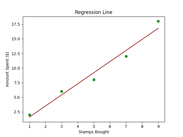
The main idea behind linear regression is to find the best-fitting straight line, the regression line, through a set of paired ( X, Y ) data. One example of the Linear Regression application is modeling the impact of flipper length on penguins’ body mass_,_ which is visualized below:

[Image Source: The Author] Regression Line showcasing best fitted line to the actual data points in the data.
Multiple Linear Regression with three independent variables can be described by the following expression:

where Y is the dependent variable, X is the independent variable which is part of the data, β0 is the intercept which is unknown and constant, and β1, β2, β3 are the slope coefficients or a parameter corresponding to the variable X1, X2, X3 which are unknown and constant as well. Finally, u is the error term that the model makes when estimating the Y values.
2.1.1 Ordinary Least Squares
The ordinary least squares (OLS) is a method for estimating the unknown parameters such as β0 and β1 in a linear regression model. The model is based on the principle of least squares that minimizes the sum of squares of the differences between the observed dependent variable and its values predicted by the linear function of the independent variable, often referred to as fitted values.
This difference between the real and predicted values of dependent variable Y is referred to as residual. What OLS does is minimize the sum of squared residuals. This optimization problem results in the following OLS estimates for the unknown parameters β0 and β1 which are also known as coefficient estimates.

Once these parameters of the Simple Linear Regression model are estimated, the fitted values of the response variable can be computed as follows:

Standard Error
The residuals or the estimated error terms can be determined as follows:

It is important to keep in mind the difference between the error terms and residuals. Error terms are never observed, while the residuals are calculated from the data. The OLS estimates the error terms for each observation but not the actual error term. So, the true error variance is still unknown.
Also, these estimates are subject to sampling uncertainty. What this means is that we will never be able to determine the exact estimate, the true value, of these parameters from sample data in an empirical application. But we can estimate it by calculating the sample residual variance.
2.1.2 OLS Assumptions
The OLS estimation method makes the following assumptions which need to be satisfied to get reliable prediction results:
Assumption (A)1: the Linearity assumption states that the model is linear in parameters.
A2: the Random Sample assumption states that all observations in the sample are randomly selected.
A3: the Exogeneity assumption states that independent variables are uncorrelated with the error terms.
A4: the Homoskedasticity assumption states that the variance of all error terms is constant.
A5: the No Perfect Multi-Collinearity assumption states that none of the independent variables is constant and there are no exact linear relationships between the independent variables.
Note that the above description for Linear Regression is from my article named Complete Guide to Linear Regression.
For detailed article on Linear Regression check out this post:
2.1.3 Linear Regression in Python
Imagine you have a friend, Alex, who collects stamps. Every month, Alex buys a certain number of stamps, and you notice that the amount Alex spends seems to depend on the number of stamps bought.
Now, you want to create a little tool that can predict how much Alex will spend next month based on the number of stamps bought. This is where Linear Regression comes into play.
In technical terms, we're trying to predict the dependent variable (amount spent) based on the independent variable (number of stamps bought).
Below is some simple Python code using scikit-learn to perform Linear Regression on a created dataset.
import numpy as np
import matplotlib.pyplot as plt
from sklearn.linear_model import LinearRegression

# Sample Data
stamps_bought = np.array([1, 3, 5, 7, 9]).reshape((-1, 1))  # Reshaping to make it a 2D array
amount_spent = np.array([2, 6, 8, 12, 18])

# Creating a Linear Regression Model
model = LinearRegression()

# Training the Model
model.fit(stamps_bought, amount_spent)

# Predictions
next_month_stamps = 10
predicted_spend = model.predict([[next_month_stamps]])

# Plotting
plt.scatter(stamps_bought, amount_spent, color='blue')
plt.plot(stamps_bought, model.predict(stamps_bought), color='red')
plt.title('Stamps Bought vs Amount Spent')
plt.xlabel('Stamps Bought')
plt.ylabel('Amount Spent ($)')
plt.grid(True)
plt.show()

# Displaying Prediction
print(f"If Alex buys {next_month_stamps} stamps next month, they will likely spend ${predicted_spend[0]:.2f}.")
Sample Data:
stamps_boughtrepresents the number of stamps Alex bought each month andamount_spentrepresents the corresponding money spent.Creating and Training Model: Using
LinearRegression()fromscikit-learnto create and train our model using.fit().Predictions: Use the trained model to predict the amount Alex will spend for a given number of stamps. In the code, we predict the amount for 10 stamps.
Plotting: We plot the original data points (in blue) and the predicted line (in red) to visually understand our model’s prediction capability.
Displaying Prediction: Finally, we print out the predicted spending for a specific number of stamps (10 in this case).
[Image Source: The Author] Visualization of Regression Line, best fitted line by LR model versus the actual data points, to see how well the model was able to fit the data.
2.2 Logistic Regression
Another very popular Machine Learning technique is Logistic Regression which, though named regression, is actually a supervised classification technique_._
Logistic regression is a Machine Learning method that models conditional probability of an event occurring or observation belonging to a certain class, based on a given dataset of independent variables.
When the relationship between two variables is linear and the dependent variable is a categorical variable, you may want to predict a variable in the form of a probability (number between 0 and 1). In these cases, Logistic Regression comes in handy.
This is because during the prediction process in Logistic Regression, the classifier predicts the probability (a value between 0 and 1) of each observation belonging to the certain class, usually to one of the two classes of dependent variable.
For instance, if you want to predict the probability or likelihood that a candidate will be elected or not during an election given the candidate's popularity score, past successes, and other descriptive variables about that candidate, you can use Logistic Regression to model this probability.
So, rather than predicting the response variable, Logistic Regression models the probability that Y belongs to a particular category.
It's similar to Linear Regression with a difference being that instead of Y it predicts the log odds. In statistical terminology, we model the conditional distribution of the response Y, given the predictor(s) X. So LR helps to predict the probability of Y belonging to certain class (0 and 1) given the features P(Y|X=x).
The name Logistic in Logistic Regression comes from the function this approach is based upon, which is Logistic Function. Logistic Function makes sure that for too large and too small values, the corresponding probability is still within the [0,1 bounds].

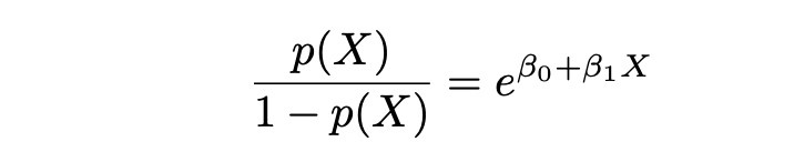
probability of observation belonging to certain class conditions on its feature value X
In the equation above, the P(X) stands for the probability of Y belonging to certain class (0 and 1) given the features P(Y|X=x). X stands for the independent variable, β0 is the intercept which is unknown and constant, β1 is the slope coefficient or a parameter corresponding to the variable X which is unknown and constant as well similar to Linear Regression. e stands for exp() function.
Odds and Log Odds
Logistic Regression and its estimation technique MLE is based on the terms Odds and Log Odds. Where Odds is defined as follows:
Odds ratio
and Log Odds is defined as follows:
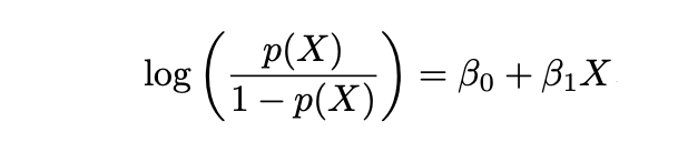
log odds ratio
2.2.1 Maximum Likelihood Estimation (MLE)
While for Linear Regression, we use OLS (Ordinary Least Squares) or LS (Least Squares) as an estimation technique, for Logistic Regression we should use another estimation technique.
We can’t use LS in Logistic Regression to find the best fitting line (to perform estimation) because the errors can then become very large or very small (even negative) while in case of Logistic Regression we aim for a predicted value in [0,1].
So for Logistic Regression we use the MLE technique, where the likelihood function calculates the probability of observing the outcome given the input data and the model. This function is then optimised to find the set of parameters that results in the largest sum likelihood over the training dataset.
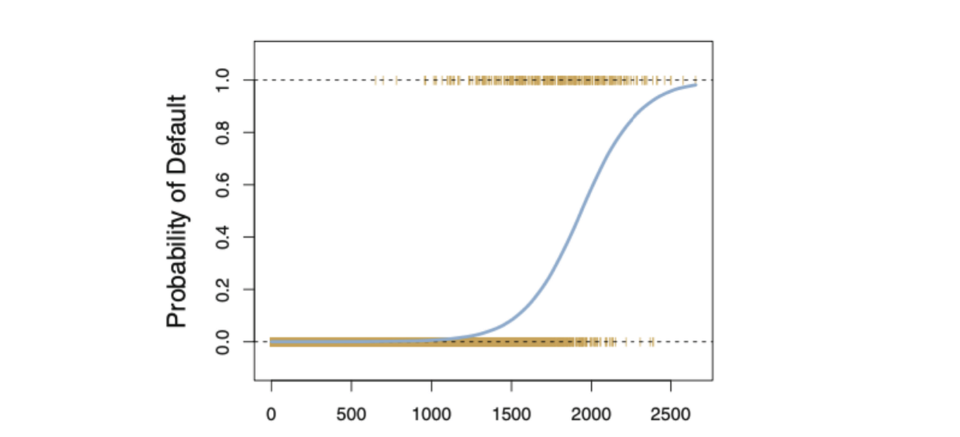
Image Source: The Author
The logistic function will always produce an S-shaped curve like above, regardless of the value of independent variable X resulting in sensible estimation most of the time.
2.2.2 Logistic Regression Likelihood Function(s)
The Likelihood function can be expressed as follows:

So the Log Likelihood function can be expressed as follows:

or, after transformation from multipliers to summation, we get:

Then the idea behind the MLE is to find a set of estimates that would maximize this likelihood function.
Step 1: Project the data points into a candidate line that produces a sample log (odds) value.
Step 2: Transform sample log (odds) to sample probabilities by using the following formula:

Step 3: Obtain the overall likelihood or overall log likelihood.
Step 4: Rotate the log (odds) line again and again, until you find the optimal log (odds) maximizing the overall likelihood
2.2.3 Cut off value in Logistic Regression
If you plan to use Logistic Regression at the end get a binary {0,1} value, then you need a cut-off point to transform the estimated values per observation from the range of [0,1] to a value 0 or 1.
Depending on your individual case you can choose a corresponding cut off point, but a popular cut-ff point is 0.5. In this case, all observations with a predicted value smaller than 0.5 will be assigned to class 0 and observations with a predicted value larger or equal than 0.5 will be assigned to class 1.
2.2.4 Performance Metrics in Logistic Regression
Since Logistic Regression is a classification method, common classification metrics such as recall, precision, F-1 measure can all be used. But there is also a metrics system that is also commonly used for assessing the performance of the Logistic Regression model, called Deviance.
2.2.5 Logistic Regression in Python
Jenny is an avid book reader. Jenny reads books of different genres and maintains a little journal where she notes down the number of pages and whether she liked the book (Yes or No).
We see a pattern: Jenny typically enjoys books that are neither too short nor too long. Now, can we predict whether Jenny will like a book based on its number of pages? This is where Logistic Regression can help us!
In technical terms, we're trying to predict a binary outcome (like/dislike) based on one independent variable (number of pages).
Here's a simplified Python example using scikit-learn to implement Logistic Regression:
import numpy as np
import matplotlib.pyplot as plt
from sklearn.linear_model import LogisticRegression
from sklearn.metrics import accuracy_score

# Sample Data
pages = np.array([100, 150, 200, 250, 300, 350, 400, 450, 500]).reshape(-1, 1)
likes = np.array([0, 1, 1, 1, 0, 0, 0, 0, 0])  # 1: Like, 0: Dislike

# Creating a Logistic Regression Model
model = LogisticRegression()

# Training the Model
model.fit(pages, likes)

# Predictions
predict_book_pages = 260
predicted_like = model.predict([[predict_book_pages]])

# Plotting
plt.scatter(pages, likes, color='forestgreen')
plt.plot(pages, model.predict_proba(pages)[:, 1], color='darkred')
plt.title('Book Pages vs Like/Dislike')
plt.xlabel('Number of Pages')
plt.ylabel('Likelihood of Liking')
plt.axvline(x=predict_book_pages, color='green', linestyle='--')
plt.axhline(y=0.5, color='grey', linestyle='--')
plt.show()

# Displaying Prediction
print(f"Jenny will {'like' if predicted_like[0] == 1 else 'not like'} a book of {predict_book_pages} pages.")
Sample Data:
pagesrepresents the number of pages in the books Jenny has read, andlikesrepresents whether she liked them (1 for like, 0 for dislike).Creating and Training Model: We instantiate
LogisticRegression()and train the model using.fit()with our data.Predictions: We predict whether Jenny will like a book with a particular number of pages (260 in this example).
Plotting: We visualize the original data points (in blue) and the predicted probability curve (in red). The green dashed line represents the page number we’re predicting for, and the grey dashed line indicates the threshold (0.5) above which we predict a "like".
Displaying Prediction: We output whether Jenny will like a book of the given page number based on our model's prediction.
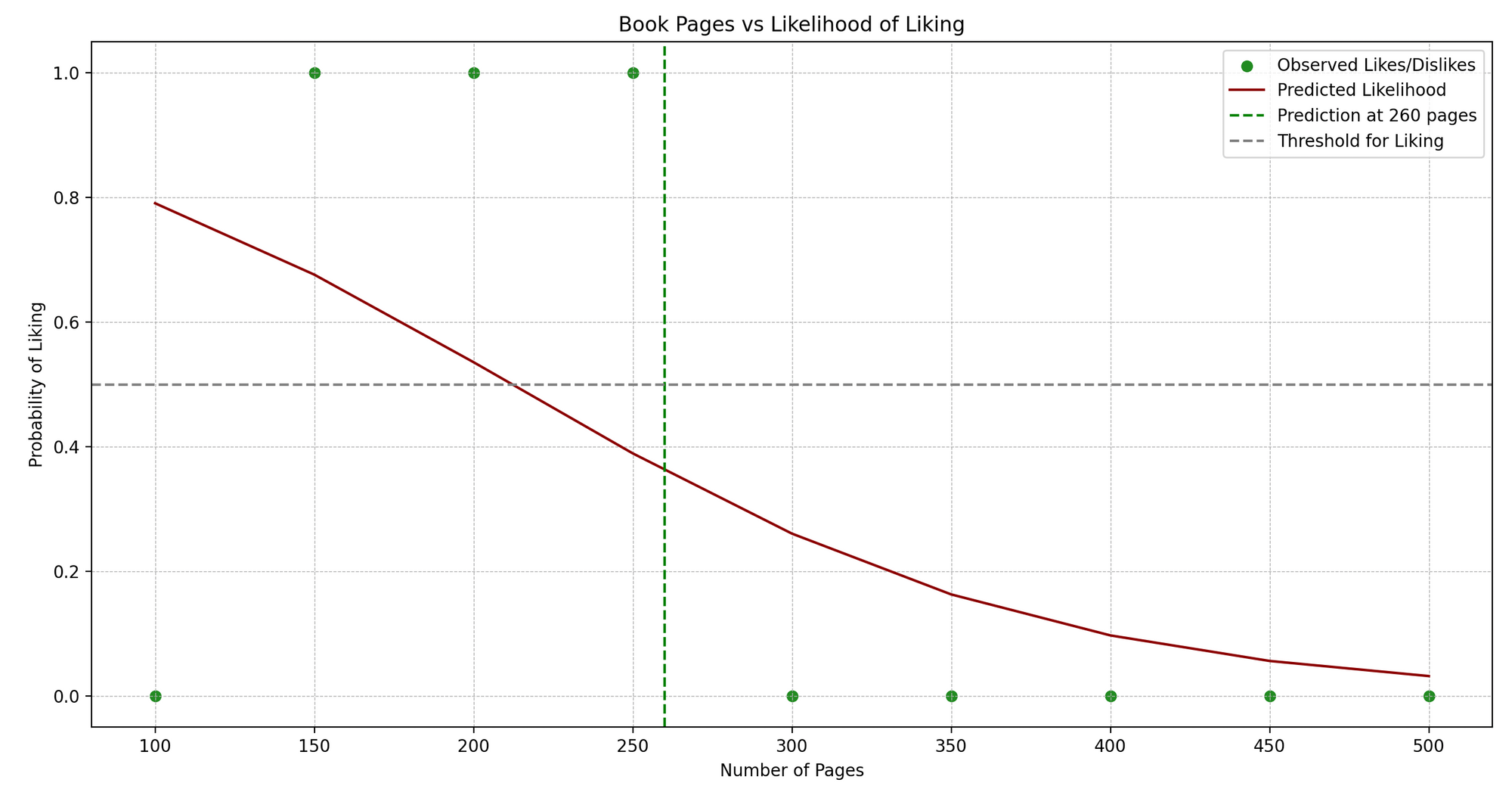
[Image Source: The Author] Visualizalization of Logisitc Regression Classification model, you can see the probability of liking given number of pages of the book, here the cut-off point is 0.5
2.3 Linear Discriminant Analysis (LDA)
Another classification technique, closely related to Logistic Regression, is Linear Discriminant Analytics (LDA). Where Logistic Regression is usually used to model the probability of observation belonging to a class of the outcome variable with 2 categories, LDA is usually used to model the probability of observation belonging to a class of the outcome variable with 3 and more categories.
LDA offers an alternative approach to model the conditional likelihood of the outcome variable given that set of predictors that addresses the issues of Logistic Regression. It models the distribution of the predictors X separately in each of the response classes (that is, given Y ), and then uses Bayes’ theorem to flip these two around into estimates for Pr(Y = k|X = x).
Note that in the case of LDA these distributions are assumed to be normal. It turns out that the model is very similar in form to logistic regression. In the equation here:

π_k represents the overall prior probability that a randomly chosen observation comes from the k_th_ class. f_k(x) , which is equal to Pr(X = x|Y = k), represents the posterior probability, and is the density function of X for an observation that comes from the k_th_ class (density function of the predictors).
This is the probability of X=x given the observation is from certain class. Stated differently, it is the probability that the observation belongs to the k_th_ class, given the predictor value for that observation.
Assuming that f_k(x) is Normal or Gaussian, the normal density takes the following form (this is the one- normal dimensional setting):


where μ_k and σ_k² are the mean and variance parameters for the k_th_ class. Assuming that σ_¹² = · · · = σ_K² (there is a shared variance term across all K classes, which we denote by σ2).
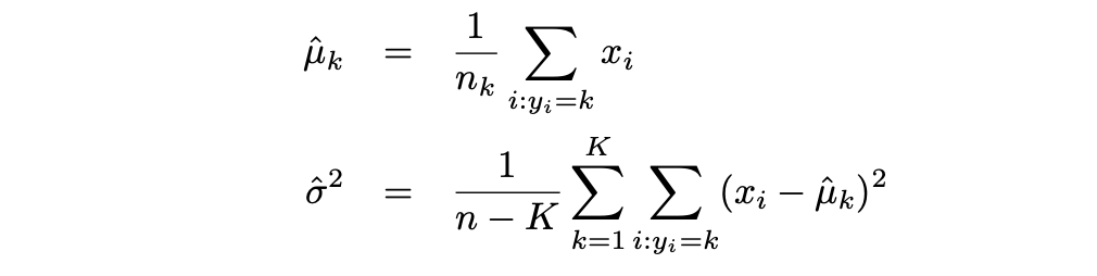
Then the LDA approximates the Bayes classifier by using the following estimates for πk, μk, and σ2:
Where Logistic Regression is usually used to model the probability of observation belonging to a class of the outcome variable with 2 categories, LDA is usually used to model the probability of observation belonging to a class of the outcome variable with 3 and more categories.
2.3.1 Linear Discriminant Analysis in Python
Imagine Sarah, who loves cooking and trying various fruits. She sees that the fruits she likes are typically of specific sizes and sweetness levels.
Now, Sarah is curious: can she predict whether she will like a fruit based on its size and sweetness? Let's use Linear Discriminant Analysis (LDA) to help her predict whether she'll like certain fruits or not.
In technical language, we are trying to classify the fruits (like/dislike) based on two predictor variables (size and sweetness).
import numpy as np
import matplotlib.pyplot as plt
from sklearn.discriminant_analysis import LinearDiscriminantAnalysis

# Sample Data
# [size, sweetness]
fruits_features = np.array([[3, 7], [2, 8], [3, 6], [4, 7], [1, 4], [2, 3], [3, 2], [4, 3]])
fruits_likes = np.array([1, 1, 1, 1, 0, 0, 0, 0])  # 1: Like, 0: Dislike

# Creating an LDA Model
model = LinearDiscriminantAnalysis()

# Training the Model
model.fit(fruits_features, fruits_likes)

# Prediction
new_fruit = np.array([[2.5, 6]])  # [size, sweetness]
predicted_like = model.predict(new_fruit)

# Plotting
plt.scatter(fruits_features[:, 0], fruits_features[:, 1], c=fruits_likes, cmap='viridis', marker='o')
plt.scatter(new_fruit[:, 0], new_fruit[:, 1], color='darkred', marker='x')
plt.title('Fruits Enjoyment Based on Size and Sweetness')
plt.xlabel('Size')
plt.ylabel('Sweetness')
plt.show()

# Displaying Prediction
print(f"Sarah will {'like' if predicted_like[0] == 1 else 'not like'} a fruit of size {new_fruit[0, 0]} and sweetness {new_fruit[0, 1]}.")
Sample Data:
fruits_featurescontains two features – size and sweetness of fruits, andfruits_likesrepresents whether Sarah likes them (1 for like, 0 for dislike).Creating and Training Model: We instantiate
LinearDiscriminantAnalysis()and train it using.fit()with our sample data.Prediction: We predict whether Sarah will like a fruit with a particular size and sweetness level ([2.5, 6] in this example).
Plotting: We visualize the original data points, color-coded based on Sarah’s like (yellow) and dislike (purple), and mark the new fruit with a red 'x'.
Displaying Prediction: We output whether Sarah will like a fruit with the given size and sweetness level based on our model's prediction.
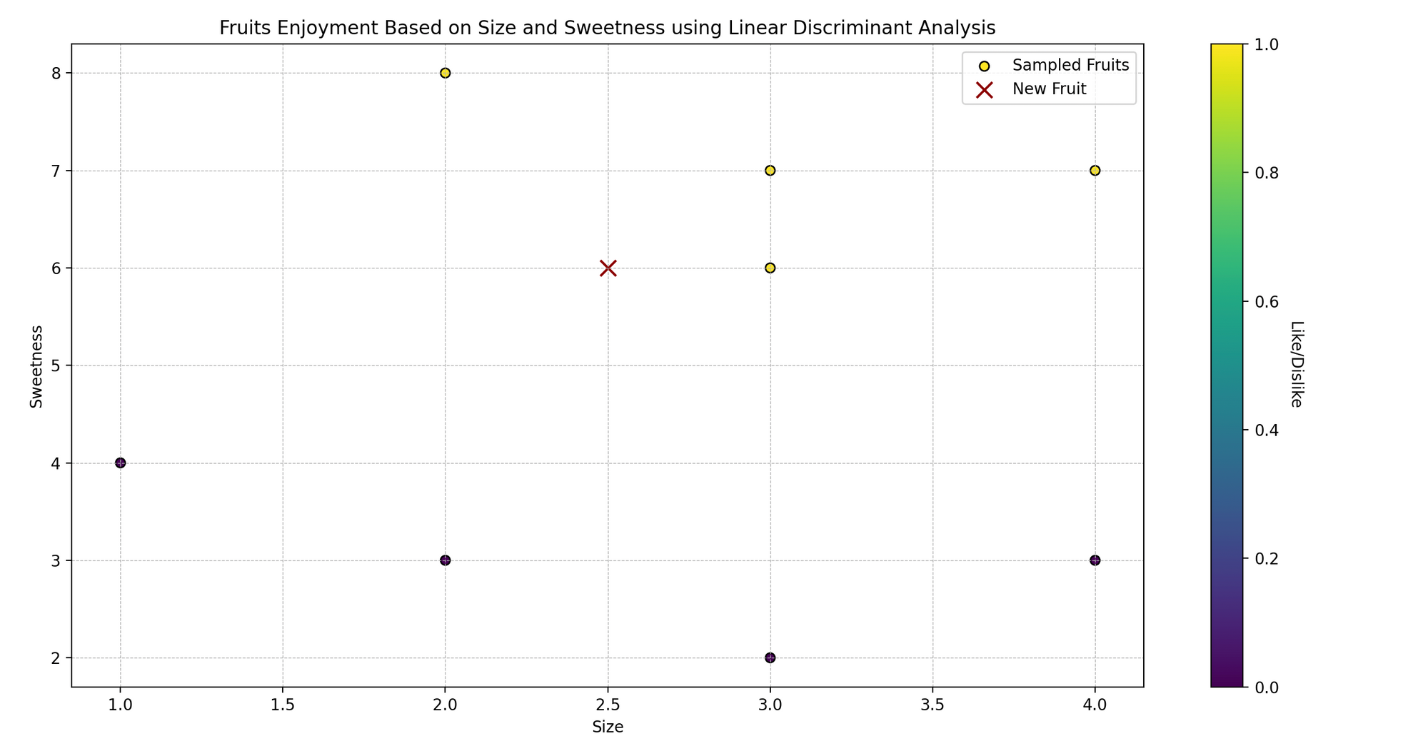
[Image Source: The Author] Graph showing the classification results of fruits, whether Sarah likes or deslikes the fruit based on fruits size and sweetness level
2.4 Logistic Regression vs LDA
Logistic regression is a popular approach for performing classification when there are two classes. But when the classes are well-separated or the number of classes exceeds 2, the parameter estimates for the logistic regression model are surprisingly unstable.
Unlike Logistic Regression, LDA does not suffer from this instability problem when the number of classes is more than 2. If n is small and the distribution of the predictors X is approximately normal in each of the classes, LDA is again more stable than the Logistic Regression model.
2.5 Naïve Bayes
Another classification method that relies on Bayes Rule**,** like LDA, is Naïve Bayes Classification approach. For more about Bayes Theorem, Bayes Rule and a corresponding example, you can read these articles.
Like Logistic Regression, you can use the Naïve Bayes approach to classify observation in one of the two classes (0 or 1).
The idea behind this method is to calculate the probability of observation belonging to a class given the prior probability for that class and conditional probability of each feature value given for given class. That is:

where Y stands for the class of observation, k is the k_th_ class and x1, …, xn stands for feature 1 till feature n, respectively. f_k(x) = Pr(X = x|Y = k), represents the posterior probability, which like in case of LDA is the density function of X for an observation that comes from the k_th_ class (density function of the predictors).
If you compare the above expression with the one you saw for LDA, you will see some similarities.
In LDA, we make a very important and strong assumption for simplification purposes: namely, that f_k is the density function for a multivariate normal random variable with class-specific mean μ_k, and shared covariance matrix Sigma Σ.
This assumtion helps to replace the very challenging problem of estimating K p-dimensional density functions with the much simpler problem, which is to estimate K p-dimensional mean vectors and one (p × p)-dimensional covariance matrices.
In the case of the Naïve Bayes Classifier, it uses a different approach for estimating f_1 (x), . . . , f_K(x). Instead of making an assumption that these functions belong to a particular family of distributions (for example normal or multivariate normal), we instead make a single assumption: within the k_th_ class, the p predictors are independent. That is:

So Bayes classifier assumes that the value of a particular variable or feature is independent of the value of any other variables (uncorrelated), given the class/label variable.
For instance, a fruit may be considered to be a banana if it is yellow, oval shaped, and about 5–10 cm long. So, the Naïve Bayes classifier considers that each of these various features of fruit contribute independently to the probability that this fruit is a banana, independent of any possible correlation between the colour, shape, and length features.
Naïve Bayes Estimation
Like Logistic Regression, in the case of the Naïve Bayes classification approach we use Maximum Likelihood Estimation (MLE) as estimation technique. There is a great article providing detailed, coincise summary for this approach with corresponding example which you can find here.
2.5.1 Naïve Bayes in Python
Tom is a movie enthusiast who watches films across different genres and records his feedback—whether he liked them or not. He has noticed that whether he likes a film might depend on two aspects: the movie's length and its genre. Can we predict whether Tom will like a movie based on these two characteristics using Naïve Bayes?
Technically, we want to predict a binary outcome (like/dislike) based on the independent variables (movie length and genre).
import numpy as np
import matplotlib.pyplot as plt
from sklearn.naive_bayes import GaussianNB

# Sample Data
# [movie_length, genre_code] (assuming genre is coded as: 0 for Action, 1 for Romance, etc.)
movies_features = np.array([[120, 0], [150, 1], [90, 0], [140, 1], [100, 0], [80, 1], [110, 0], [130, 1]])
movies_likes = np.array([1, 1, 0, 1, 0, 1, 0, 1])  # 1: Like, 0: Dislike

# Creating a Naive Bayes Model
model = GaussianNB()

# Training the Model
model.fit(movies_features, movies_likes)

# Prediction
new_movie = np.array([[100, 1]])  # [movie_length, genre_code]
predicted_like = model.predict(new_movie)

# Plotting
plt.scatter(movies_features[:, 0], movies_features[:, 1], c=movies_likes, cmap='viridis', marker='o')
plt.scatter(new_movie[:, 0], new_movie[:, 1], color='darkred', marker='x')
plt.title('Movie Likes Based on Length and Genre')
plt.xlabel('Movie Length (min)')
plt.ylabel('Genre Code')
plt.show()

# Displaying Prediction
print(f"Tom will {'like' if predicted_like[0] == 1 else 'not like'} a {new_movie[0, 0]}-min long movie of genre code {new_movie[0, 1]}.")
Sample Data:
movies_featurescontains two features: movie length and genre (encoded as numbers), whilemovies_likesindicates whether Tom likes them (1 for like, 0 for dislike).Creating and Training Model: We instantiate
GaussianNB()(a Naïve Bayes classifier assuming Gaussian distribution of data) and train it with.fit()using our data.Prediction: We predict whether Tom will like a new movie, given its length and genre code ([100, 1] in this case).
Plotting: We visualize the original data points, color-coded based on Tom’s like (yellow) and dislike (purple). The red 'x' represents the new movie.
Displaying Prediction: We print whether Tom will like a movie of the given length and genre code, as per our model's prediction.
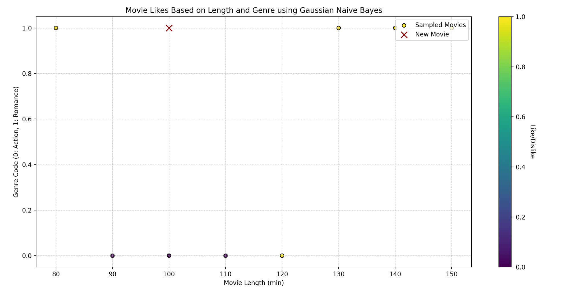
[Image Source: The Author] Movie likes based on length and genre using Gaussian Naïve Bayes
2.6 Naïve Bayes vs Logistic Regression
Naïve Bayes Classifier has proven to be faster and has a higher bias and lower variance. Logistic regression has a low bias and higher variance. Depending on your individual case, and the bias-variance trade-off, you can pick the corresponding approach.
2.7 Decision Trees
Decision Trees are a supervised and non-parametric Machine Learning learning method used for both classification and regression purposes. The idea is to create a model that predicts the value of a target variable by learning simple decision rules from the data predictors.
Unlike Linear Regression, or Logistic Regression, Decision Trees are simple and useful model alternatives when the relationship between independent variables and dependent variable is suspected to be non-linear.
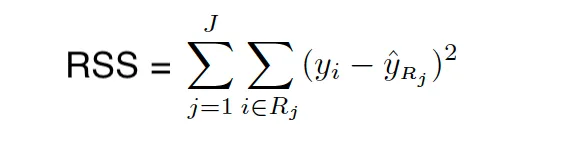
Tree-based methods stratify or segment the predictor space into smaller regions. The idea behind building Decision Trees is to divide the predictor space into distinct and mutually exclusive regions X1,X2,….. ,Xp → R_1,R_2, …,R_N where the regions are in the form of boxes or rectangles. These regions are found by recursive binary splitting since minimizing the RSS is not feasible. This approach is often referred to as a greedy approach.
Decision trees are built by top-down splitting. So, in the beginning, all observations belong to a single region. Then, the model successively splits the predictor space. Each split is indicated via two new branches further down on the tree.
This approach is sometimes called greedy because at each step of the tree-building process, the best split is made at that particular step, rather than looking ahead and picking a split that will lead to a better tree in some future step.
Stopping Criteria
There are some common stopping criteria used when building Decision Trees:
Minimum number of observations in the leaf.
Minimum number of samples for a node split.
Maximum depth of tree (vertical depth).
Maximum number of terminal nodes.
Maximum features to consider for the split.
For example, repeat this splitting process until no region contains more than 100 observations. Let's dive deeper
**1. Minimum number of observations in the leaf:**If a proposed split results in a leaf node with fewer than a defined number of observations, that split might be discarded. This prevents the tree from becoming overly complex.
**2. Minimum number of samples for a node split:**To proceed with a node split, the node must have at least this many samples. This ensures that there's a significant amount of data to justify the split.
**3. Maximum depth of tree (vertical depth):**This limits how many times a tree can split. It's like telling the tree how many questions it can ask about the data before making a decision.
**4. Maximum number of terminal nodes:**This is the total number of end nodes (or leaves) the tree can have.
**5. Maximum features to consider for the split:**For each split, the algorithm considers only a subset of features. This can speed up training and help in generalization.
When building a decision tree, especially when dealing with large number of features, the tree can become too big with too many leaves. This will effect the interpretability of the model, and might potentially result in an overfitting problem. Therefore, picking a good stopping criteria is essential for the interpretability and for the performance of the model.
RSS/Gini Index/Entropy/Node Purity
When building the tree, we use RSS (for Regression Trees) and GINI Index/Entropy (for Classification Trees) for picking the predictor and value for splitting the regions. Both Gini Index and Entropy are often called Node Purity measures because they describe how pure the leaf of the trees are.
Gini Index
The Gini index measures the total variance across K classes. It takes small value when all class error rates are either 1 or 0. This is also why it’s called a measure for node purity – Gini index takes small values when the nodes of the tree contain predominantly observations from the same class.
The Gini index is defined as follows:

where pˆmk represents the proportion of training observations in the mth region that are from the kth class.
Entropy
Entropy is another node purity measure, and like the Gini index, the entropy will take on a small value if the m_th_ node is pure. In fact, the Gini index and the entropy are quite similar numerical and can be expressed as follows:

Decision Tree Classification Example
Let’s look at an example where we have three features describing consumers' past behaviour:
Recency (How recent was the customer’s last purchase?)
Monetary (How much money did the customer spend in a given period?)
Frequency (How often did this customer make a purchase in a given period?)
We will use the classification version of the Decision Tree to classify customers to 1 of the 3 classes (Good: 1, Better: 2 and Best: 3), given the features describing the customer's behaviour.
In the following tree, where we use Gini Index as a purity measure, we see that the first features that seems to be the most important one is the Recency. Let's look at the tree and then interpret it:

[Image Source: The Author] Decision tree
Customers who have a recency of 202 or larger (last time has made a purchase > 202 days ago) then the chance of this observation to be assigned to class 1 is 93% (basically, we can label those customers as Good Class customers).
For customers with Recency less than 202 (they made a purchase recently), we look at their Monetary value and if it's smaller than 1394, then we look at their Frequency. If the Frequency is then smaller than 44, we can then label this customers’ class as Better or (class 2). And so on.
Decision Trees Python Implementation
Alex is intrigued by the relationship between the number of hours studied and the scores obtained by students. Alex collected data from his peers about their study hours and respective test scores.
He wonders: can we predict a student's score based on the number of hours they study? Let's leverage Decision Tree Regression to uncover this.
Technically, we're predicting a continuous outcome (test score) based on an independent variable (study hours).
import numpy as np
import matplotlib.pyplot as plt
from sklearn.tree import DecisionTreeRegressor, plot_tree

# Sample Data
# [hours_studied]
study_hours = np.array([1, 2, 3, 4, 5, 6, 7, 8]).reshape(-1, 1)
test_scores = np.array([50, 55, 70, 80, 85, 90, 92, 98])

# Creating a Decision Tree Regression Model
model = DecisionTreeRegressor(max_depth=3)

# Training the Model
model.fit(study_hours, test_scores)

# Prediction
new_study_hour = np.array([[5.5]])  # example of hours studied
predicted_score = model.predict(new_study_hour)

# Plotting the Decision Tree
plt.figure(figsize=(12, 8))
plot_tree(model, filled=True, rounded=True, feature_names=["Study Hours"])
plt.title('Decision Tree Regressor Tree')
plt.show()

# Plotting Study Hours vs. Test Scores
plt.scatter(study_hours, test_scores, color='darkred')
plt.plot(np.sort(study_hours, axis=0), model.predict(np.sort(study_hours, axis=0)), color='orange')
plt.scatter(new_study_hour, predicted_score, color='green')
plt.title('Study Hours vs Test Scores')
plt.xlabel('Study Hours')
plt.ylabel('Test Scores')
plt.grid(True)
plt.show()

# Displaying Prediction
print(f"Predicted test score for {new_study_hour[0, 0]} hours of study: {predicted_score[0]:.2f}.")
Sample Data:
study_hourscontains hours studied, andtest_scorescontains the corresponding test scores.Creating and Training Model: We create a
DecisionTreeRegressorwith a specified maximum depth (to prevent overfitting) and train it with.fit()using our data.Plotting the Decision Tree:
plot_treehelps visualize the decision-making process of the model, representing splits based on study hours.Prediction & Plotting: We predict the test score for a new study hour value (5.5 in this example), visualize the original data points, the decision tree’s predicted scores, and the new prediction.
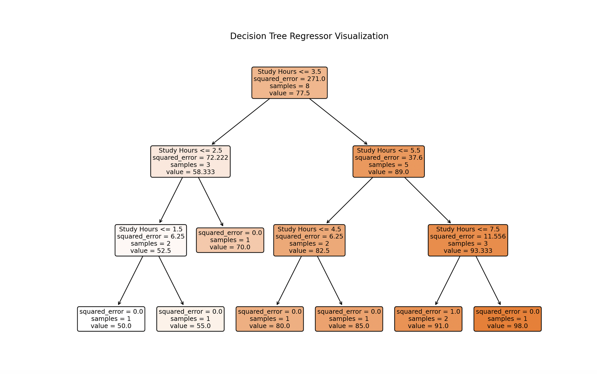
[Image Source: The Author] Decision tree regressor visualization
The visualization depicts a decision tree model trained on study hours data. Each node represents a decision based on study hours, branching from the top root based on conditions that best forecast test scores. The process continues until reaching a maximum depth or no further meaningful splits. Leaf nodes at the bottom give final predictions, which for regression trees, are the average of target values for training instances reaching that leaf. This visualization highlights the model's predictive approach and the significant influence of study hours on test scores.
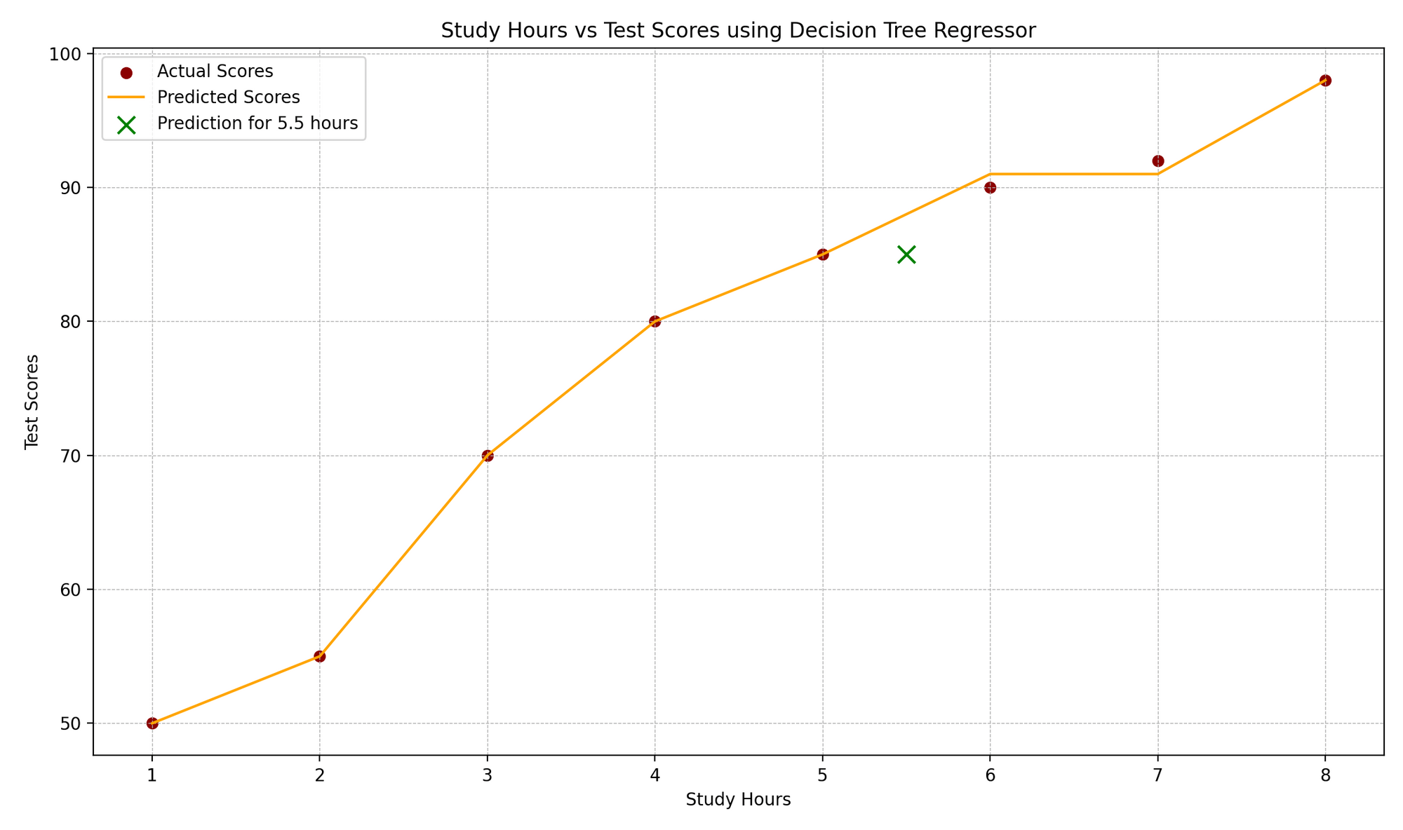
[Image Source: The Author] Study hours vs test scores plotted using decision tree regressor
The "Study Hours vs. Test Scores" plot illustrates the correlation between study hours and corresponding test scores. Actual data points are denoted by red dots, while the model's predictions are shown as an orange step function, characteristic of regression trees. A green "x" marker highlights a prediction for a new data point, here representing a 5.5-hour study duration. The plot's design elements, such as gridlines, labels, and legends, enhance comprehension of the real versus anticipated values.
2.8 Bagging
One of the biggest disadvantages of Decision Trees is their high variance. You might end up with a model and predictions that are easy to explain but misleading. This would result in making incorrect conclusions and business decisions.
So to reduce the variance of the Decision trees, you can use a method called Bagging. To understand what Bagging is, there are two terms you need to know:
Bootstrapping
Central Limit Theorem (CLT)
You can find more about Boostrapping, which is a resampling technique, later in this handbook. For now, you can think of Bootstrapping as a technique that performs sampling from the original data with replacement, which creates a copy of the data very similar to but not exactly the same as the original data.
Bagging is also based on the same ideas as the CLT which is one of the most important if not the most important theorem in Statistics. You can read in more detail about CLT [here](http://Suppose X1, X2, . . . , Xn are all independent random variables with the same underlying distribution, also called independent identically-distributed or i.i.d, where all X’s have the same mean μ and standard deviation σ. As the sample size grows, the probability distribution of X converges in the distribution in Normal distribution with mean μ and variance σ-squared. The Central Limit Theorem can be summarized as follows:).
But the idea that is also used in Bagging is that if you take the average of many samples, then the variance is significantly reduced compared to the variance of each of the individual sample based models.
So, given a set of n independent observations Z1,…,Zn, each with variance σ2, the variance of the mean Z ̄ of the observations is given byσ2/n. So averaging a set of observations reduces variance.
For more Statistical details, check out the following tutorial:
Bagging is basically a Bootstrap aggregation that builds B trees using Bootrsapped samples. Bagging can be used to improve the precision (lower the variance of many approaches) by taking repeated samples from a single training data.
So, in Bagging, we generate B bootstrapped training samples, based on which B similar trees (correlated trees) are built that end up being aggregaated to calculate the predictions, so taking the average of these predictions for these B-samples. Notably, each tree is built on a bootstrap data set, independent of the other trees.
So, in case of Bagging in each tree split all p features are considered which results in similar trees wince every time the strongest predictors are at the top and weak ones at the bottom resulting all of the bagged trees will look quite similar to each other.
2.8.1 Bagging in Regression Trees
To apply bagging to regression trees, we simply construct B regression trees using B bootstrapped training sets, and average the resulting predictions. These trees are grown deep, and are not pruned. So each individual tree has high variance, but low bias. Averaging these B trees reduces the variance.
2.8.2 Bagging in Classification Trees
For a given test observation, we can record the class predicted by each of the B trees, and take a majority vote: the overall prediction is the most commonly occurring majority class among the B predictions.
2.8.3 OOB Out-of-Bag Error Estimation
When Bagging is applied to decision trees, there is no longer a need to apply Cross Validation to estimate the test error rate. In bagging, we repeatedly fit the trees to Bootstrapped samples – and on average only 2/3 of these observations are used. The other 1/3 are not used during the training process. These are called Out-of-bag observations.
So there are in total B/3 prediction per ith observation not used in training. We can take the average of response values for these cases (or majority class). So per observation, the OOB error and average of these forms the test error rate.
2.8.4 Bagging in Python
Meet Lucy, a fitness coach who is curious about predicting her clients’ weight loss based on their daily calorie intake and workout duration. Lucy has data from past clients but recognizes that individual predictions might be prone to errors. Let's utilize Bagging to create a more stable prediction model.
Technically, we'll predict a continuous outcome (weight loss) based on two independent variables (daily calorie intake and workout duration), using Bagging to reduce variance in predictions.
import numpy as np
import matplotlib.pyplot as plt
from sklearn.ensemble import BaggingRegressor
from sklearn.tree import DecisionTreeRegressor, plot_tree  # Ensure plot_tree is imported
from sklearn.model_selection import train_test_split
from sklearn.metrics import mean_squared_error

# Sample Data
clients_data = np.array([[2000, 60], [2500, 45], [1800, 75], [2200, 50], [2100, 62], [2300, 70], [1900, 55], [2000, 65]])
weight_loss = np.array([3, 2, 4, 3, 3.5, 4.5, 3.7, 4.2])

# Train-Test Split
X_train, X_test, y_train, y_test = train_test_split(clients_data, weight_loss, test_size=0.25, random_state=42)

# Creating a Bagging Model
base_estimator = DecisionTreeRegressor(max_depth=4)
model = BaggingRegressor(base_estimator=base_estimator, n_estimators=10, random_state=42)

# Training the Model
model.fit(X_train, y_train)

# Prediction & Evaluation
y_pred = model.predict(X_test)
mse = mean_squared_error(y_test, y_pred)

# Displaying Prediction and Evaluation
print(f"True weight loss: {y_test}")
print(f"Predicted weight loss: {y_pred}")
print(f"Mean Squared Error: {mse:.2f}")

# Visualizing One of the Base Estimators (if desired)
plt.figure(figsize=(12, 8))
tree = model.estimators_[0]
plt.title('One of the Base Decision Trees from Bagging')
plot_tree(tree, filled=True, rounded=True, feature_names=["Calorie Intake", "Workout Duration"])
plt.show()
True weight loss: [2. 4.5]
Predicted weight loss: [3.1 3.96]
Mean Squared Error: 0.75
Sample Data:
clients_datacontains daily calorie intake and workout duration, andweight_losscontains the corresponding weight loss.Train-Test Split: We split the data into training and test sets to validate the model's predictive performance.
Creating and Training Model: We instantiate
BaggingRegressorwithDecisionTreeRegressoras the base estimator and train it using.fit()with our training data.Prediction & Evaluation: We predict weight loss for the test data, evaluating prediction quality with Mean Squared Error (MSE).
Visualizing One of the Base Estimators: Optionally, visualize one tree from the ensemble to understand individual decision-making processes (keeping in mind an individual tree may not perform well, but collectively they produce stable predictions).
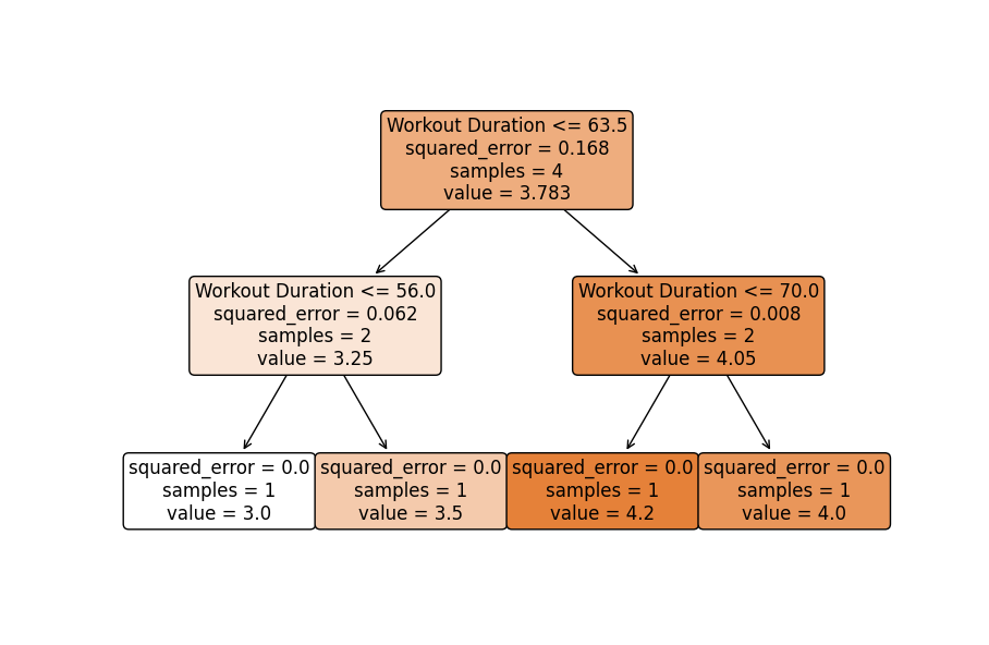
Image Source: The Author (this is one of the decision trees in Bagging)
2.9 Random Forest
Random forests provide an improvement over bagged trees by way of a small tweak that decorrelates the trees.
As in bagging, we build a number of decision trees on bootstrapped training samples. But when building these decision trees, each time a split in a tree is considered, a random sample of m predictors is chosen as split candidates from the full set of p predictors.
The split is allowed to use only one of those m predictors. A fresh and random sample of m predictors is taken at each split, and typically we choose m ≈ √p — that is, the number of predictors considered at each split is approximately equal to the square root of the total number of predictors. This is also the reason why Random Forest is called “random”.
The main difference between bagging and random forests is the choice of predictor subset size m decorrelates the trees.
Using a small value of m in building a random forest will typically be helpful when we have a large number of correlated predictors. So, if you have a problem of Multicollearity, RF is a good method to fix that problem.
So, unlike in Bagging, in the case of Random Forest, in each tree split not all p predictors are considered – but only randomly selected m predictors from it. This results in not similar trees being decorrelateed. And due to the fact that averaging decorrelated trees results in smaller variance, Random Forest is more accurate than Bagging.
2.9.1 Random Forest Python Implementation
Noah is a botanist who has collected data about various plant species and their characteristics, such as leaf size and flower color. Noah is curious if he could predict a plant’s species based on these features.
Here, we’ll utilize Random Forest, an ensemble learning method, to help him classify plants.
Technically, we aim to classify plant species based on certain predictor variables using a Random Forest model.
import numpy as np
import matplotlib.pyplot as plt
from sklearn.ensemble import RandomForestClassifier
from sklearn.model_selection import train_test_split
from sklearn.metrics import classification_report

# Expanded Data
plants_features = np.array([
    [3, 1], [2, 2], [4, 1], [3, 2], [5, 1], [2, 2], [4, 1], [5, 2],
    [3, 1], [4, 2], [5, 1], [3, 2], [2, 1], [4, 2], [3, 1], [4, 2],
    [5, 1], [2, 2], [3, 1], [4, 2], [2, 1], [5, 2], [3, 1], [4, 2]
])
plants_species = np.array([
    0, 1, 0, 1, 0, 1, 0, 1,
    0, 1, 0, 1, 0, 1, 0, 1,
    0, 1, 0, 1, 0, 1, 0, 1
])

# Train-Test Split
X_train, X_test, y_train, y_test = train_test_split(plants_features, plants_species, test_size=0.25, random_state=42)

# Creating a Random Forest Model
model = RandomForestClassifier(n_estimators=10, random_state=42)

# Training the Model
model.fit(X_train, y_train)

# Prediction & Evaluation
y_pred = model.predict(X_test)
classification_rep = classification_report(y_test, y_pred)

# Displaying Prediction and Evaluation
print("Classification Report:")
print(classification_rep)


# Scatter Plot Visualizing Classes
plt.figure(figsize=(8, 4))
for species, marker, color in zip([0, 1], ['o', 's'], ['forestgreen', 'darkred']):
    plt.scatter(plants_features[plants_species == species, 0],
                plants_features[plants_species == species, 1],
                marker=marker, color=color, label=f'Species {species}')
plt.xlabel('Leaf Size')
plt.ylabel('Flower Color (coded)')
plt.title('Scatter Plot of Species')
plt.legend()
plt.tight_layout()
plt.show()

# Visualizing Feature Importances
plt.figure(figsize=(8, 4))
features_importance = model.feature_importances_
features = ["Leaf Size", "Flower Color"]
plt.barh(features, features_importance, color = "darkred")
plt.xlabel('Importance')
plt.ylabel('Feature')
plt.title('Feature Importance')
plt.show()
Sample Data:
plants_featurescontains leaf size and flower color, whileplants_speciesindicates the species of the respective plant.Train-Test Split: We separate the data into training and test sets.
Creating and Training Model: We instantiate
RandomForestClassifierwith a specified number of trees (10 in this case) and train it using.fit()with our training data.Prediction & Evaluation: We predict the species for the test data and evaluate the predictions using a classification report which provides precision, recall, f1-score, and support.
Visualizing Feature Importances: We utilize a horizontal bar chart to display the importance of each feature in predicting the plant species. Random Forest quantifies the usefulness of features during the tree-building process, which we visualize here.
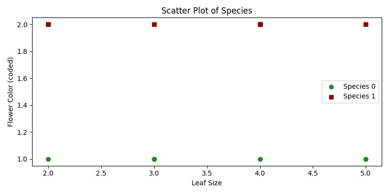
[Image Source: The Author] Scatter plot of species
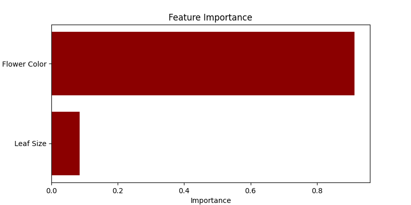
[Image Source: The Author] you can see that Flower Color feature has the largest impact in determining plant species.
2.10 Boosting or Ensemble Models
Like Bagging (averaging correlated Decision Trees) and Random Forest (averaging uncorrelated Decision Trees), Boosting aims to improve the predictions resulting from a decision tree. Boosting is a supervised Machine Learning model that can be used for both regression and classification problems.
Unlike Bagging or Random Forest, where the trees are built independently from each other using one of the B bootstrapped samples (copy of the initial training date), in Boosting, the trees are built sequentially and dependent on each other. Each tree is grown using information from previously grown trees.
Boosting does not involve bootstrap sampling. Instead, each tree fits on a modified version of the original data set. It’s a method of converting weak learners into strong learners.
In boosting, each new tree is a fit on a modified version of the original data set. So, unlike fitting a single large decision tree to the data, which amounts to fitting the data hard and potentially overfitting, the boosting approach instead learns slowly.
Given the current model, we fit a decision tree to the residuals from the model. That is, we fit a tree using the current residuals, rather than the outcome Y, as the response. We then add this new decision tree into the fitted function in order to update the residuals.
Each of these trees can be rather small, with just a few terminal nodes, determined by the parameter d in the algorithm. Now let's have a look at 3 most popular Boosting models in Machine Learning:
AdaBoost
GBM
XGBoost
2.10.1 Boosting: AdaBoost
The first Ensemble algorithm we will look into today is AdaBoost. Like in all boosting techniques, in the case of AdaBoost the trees are built using the information from the previous tree – and more specifically part of the tree which didn’t perform well. This is called the weak learner (Decision Stump). This Decision Stump is built using only a single predictor and not all predictors to perform the prediction.
So, AdaBoost combines weak learners to make classifications and each stump is made by using the previous stump’s errors. Here is the step-by-step plan for building an AdaBoost model:
Step 1: Initial Weight Assignment – assign equal weight to all observations in the sample where this weight represents the importance of the observations being correctly classified: 1/N (all samples are equally important at this stage).
Step 2: Optimal Predictor Selection – The first stamp is built by obtaining the RSS (in case of regression) or GINI Index/Entropy (in case of classification) for each predictor. Picking the stump that does the best job in terms of prediction accuracy: the stump with the smallest RSS or GINI/Entropy is selected as the next tree.
Step 3: Computing Stumps Weight based on Stumps Total Error – The importance of this stump in the final tree is then determined using the total error that this stump is making. Where a stump that is not better than random flip of a coin with total error equal to 0.5 gets weight 0. Weight = 0.5*log(1-Total Error/Total Error)
Step 4: Updating Observation Weights – We increase the weight of the observations which have been incorrectly predicted and decrease the remaining observations which had higher accuracy or have been correctly classified, so that the next stump will have higher importance of correctly predicted the value f this observation.
Step 5: Building the next Stump based on updated weights – Using Weighted Gini index to chose the next stump.
Step 6: Combining B stumps – Then all the stumps are combined while taking into account their importance, weighted sum.
AdaBoost Python Implementation
Imagine a scenario where we aim to predict house prices based on certain features like the number of rooms and age of the house.
For this example, let's generate synthetic data where: num_rooms: The number of rooms in the house. house_age: The age of the house in years. price: The price of the house in thousand dollars:
import numpy as np
import pandas as pd
import matplotlib.pyplot as plt
from sklearn.model_selection import train_test_split
from sklearn.ensemble import AdaBoostRegressor
from sklearn.metrics import mean_squared_error

# Seed for reproducibility
np.random.seed(42)

# Generate synthetic data
num_samples = 200
num_rooms = np.random.randint(3, 10, num_samples)
house_age = np.random.randint(1, 100, num_samples)
noise = np.random.normal(0, 50, num_samples)

# Assume a linear relation with price = 50*rooms + 0.5*age + noise
price = 50*num_rooms + 0.5*house_age + noise

# Create DataFrame
data = pd.DataFrame({'num_rooms': num_rooms, 'house_age': house_age, 'price': price})

# Plot
plt.scatter(data['num_rooms'], data['price'], label='Num Rooms vs Price', color = 'forestgreen')
plt.scatter(data['house_age'], data['price'], label='House Age vs Price', color = 'darkred')
plt.xlabel('Feature Value')
plt.ylabel('Price')
plt.legend()
plt.title('Scatter Plots of Features vs Price')
plt.show()

# Splitting data into training and testing sets
X = data[['num_rooms', 'house_age']]
y = data['price']
X_train, X_test, y_train, y_test = train_test_split(X, y, test_size=0.2, random_state=42)

# Initialize and train AdaBoost Regressor model
model_ab = AdaBoostRegressor(n_estimators=100, random_state=42)
model_ab.fit(X_train, y_train)

# Predictions
predictions = model_ab.predict(X_test)

# Evaluate the model
mse = mean_squared_error(y_test, predictions)
rmse = np.sqrt(mse)
print(f"Mean Squared Error: {mse:.2f}")
print(f"Root Mean Squared Error: {rmse:.2f}")

# Visualization: Actual vs Predicted Prices
plt.scatter(y_test, predictions, color = 'darkred')
plt.plot([y_test.min(), y_test.max()], [y_test.min(), y_test.max()], 'k--', lw=3)
plt.xlabel('Actual Prices')
plt.ylabel('Predicted Prices')
plt.title('Actual vs Predicted House Prices with AdaBoost')
plt.show()

[Image Source: The Author] Scatter plot of features vs price
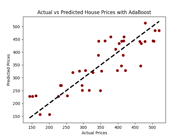
[Image Source: The Author] Actual vs predicted house prices with AdaBoost
2.10.2 Boosting Algorithm: Gradient Boosting Model (GBM)
AdaBoost and Gradient Boosting are very similar to each other. But compared to AdaBoost, which starts the process by selecting a stump and continuing to build it by using the weak learners from the previous stump, Gradient Boosting starts with a single leaf instead of a tree of a stump.
The outcome corresponding to this chosen leaf is then an initial guess for the outcome variable. Like in the case of AdaBoost, Gradient Boosting uses the previous stump’s errors to build the tree. But unlike in AdaBoost, the trees that Gradient Boost builds are larger than a stump. That’s a parameter where we set a max number of leaves.
To make sure the tree is not overfitting, Gradient Boosting uses the Learning Rate to scale the gradient contributions. Gradient Boosting is based on the idea that taking lots of small steps in the right direction (gradients) will result in lower variance (for testing data).
The major difference between the AdaBoost and Gradient Boosting algorithms is how the two identify the shortcomings of weak learners (for example, decision trees). While the AdaBoost model identifies the shortcomings by using high weight data points, gradient boosting performs the same by using gradients in the loss function (y=ax+b+e , e needs a special mention as it is the error term).
The loss function is a measure indicating how good a model’s coefficients are at fitting the underlying data. A logical understanding of loss function would depend on what we are trying to optimise.
Early Stopping
The special process of tuning the number of iterations for an algorithm (such as GBM and Random Forest) is called “Early Stopping” – a phenomenon we touched upon when discussing the Decision Trees.
Early Stopping performs model optimisation by monitoring the model’s performance on a separate test data set and stopping the training procedure once the performance on the test data stops improving beyond a certain number of iterations.
It avoids overfitting by attempting to automatically select the inflection point where performance on the test dataset starts to decrease while performance on the training dataset continues to improve as the model starts to overfit.
In the context of GBM, early stopping can be based either on an out of bag sample set (“OOB”) or cross-validation (“CV”). Like mentioned earlier, the ideal time to stop training the model is when the validation error has decreased and started to stabilise before it starts increasing due to overfitting.
To build GBM, follow this step-by-step process:
Step 1: Train the model on the existing data to predict the outcome variable
Step 2: Compute the error rate using the predictions and the real values (Pseudo Residual)
Step 3: Use the existing features and the Pseudo Residual as the outcome variable to predict the residuals again
Step 4: Use the predicted residuals to update the predictions from the Step 1, while scaling this contribution to the tree with a learning rate (hyper parameter)
Step 5: Repeat steps 1–4, the process of updating the pseudo residuals and the tree while scaling with the learning rate, to move slowly in the right direction until there is no longer an improvement or we come to our stopping rule
The idea is that each time we add a new scaled tree to the model, the residuals should get smaller.
At any m step, the Gradient Boosting model produces a model that is an ensemble of the previous step F(m-1) and learning rate eta multiplied with the negative derivative of the loss function with regard to the output of the model at step m-1: (weak learner at step m-1).

GBM Python Implementation
# Initialize and train Gradient Boosting Regressor model
model_gbm = GradientBoostingRegressor(n_estimators=100, learning_rate=0.1, max_depth=1, random_state=42)
model_gbm.fit(X_train, y_train)

# Predictions
predictions = model_gbm.predict(X_test)

# Evaluate the model
mse = mean_squared_error(y_test, predictions)
rmse = np.sqrt(mse)
print(f"Mean Squared Error: {mse:.2f}")
print(f"Root Mean Squared Error: {rmse:.2f}")

# Visualization: Actual vs Predicted Prices
plt.scatter(y_test, predictions, color = 'orange')
plt.plot([y_test.min(), y_test.max()], [y_test.min(), y_test.max()], 'k--', lw=3)
plt.xlabel('Actual Prices')
plt.ylabel('Predicted Prices')
plt.title('Actual vs Predicted House Prices with GBM')
plt.show()

[Image Source: The Author] Actual vs predicted house prices with GBM
2.10.3 Boosting Algorithm: XGBoost
One of the most popular Boosting or Ensemble algorithms is Extreme Gradient Boosting (XGBoost).
The difference between the GBM and XGBoost is that in case of XGBoost the second-order derivatives are calculated (second-order gradients). This provides more information about the direction of gradients and how to get to the minimum of the loss function.
Remember that this is needed to identify the weak learner and improve the model by improving the weak learners.
The idea behind the XGBoost is that the 2nd order derivative tends to be more precise in terms of finding the accurate direction. Like the AdaBoost, XGBoost applies advanced regularization in the form of L1 or L2 norms to address overfitting.
Unlike the AdaBoost, XGBoost is parallelizable due to its special cashing mechanism, making it convenient to handle large and complex datasets. Also, to speed up the training, XGBoost uses an Approximate Greedy Algorithm to consider only limited amount of tresholds for splitting the nodes of the trees.
To build an XGBoost model, follow this step-by-step process:
Step 1: Fit a Single Decision Tree – In this step, the Loss function is calculated, for example NDCG to evaluate the model.
Step 2: Add the Second Tree – This is done such that when this second tree is added to the model, it lowers the Loss function based on 1st and 2nd order derivatives compared to the previous tree (where we also used learning rate eta).
Step 3: Finding the Direction of the Next Move – Using the first degree and second-degree derivatives, we can find the direction in which the Loss function decreases the largest. This is basically the gradient of the Loss function with regard to to the output of the previous model.
Step 4: Splitting the nodes – To split the observations, XGBoost uses Approximate Greedy Algorithm (about 3 approximate weighted quantiles usually) quantiles that have a similar sum of weights. For finding the split value of the nodes, it doesn't consider all the candidate thresholds but instead it uses the quantiles of that predictor only.
Optimal Learning Rate can be determined by using Cross Validation & Grid Search.
Simple XGBoost Python Implementation
Imagine you have a dataset containing information about various houses and their prices. The dataset includes features like the number of bedrooms, bathrooms, the total area, the year built, and so on, and you want to predict the price of a house based on these features.
import xgboost as xgb

# Initialize and train XGBoost model
model_xgb = xgb.XGBRegressor(objective ='reg:squarederror', n_estimators = 100, seed = 42)
model_xgb.fit(X_train, y_train)

# Predictions
predictions = model_xgb.predict(X_test)

# Evaluate the model
mse = mean_squared_error(y_test, predictions)
rmse = np.sqrt(mse)
print(f"Mean Squared Error: {mse:.2f}")
print(f"Root Mean Squared Error: {rmse:.2f}")

# Visualization: Actual vs Predicted Prices
plt.scatter(y_test, predictions, color="forestgreen")
plt.plot([y_test.min(), y_test.max()], [y_test.min(), y_test.max()], 'k--', lw=3)
plt.xlabel('Actual Prices')
plt.ylabel('Predicted Prices')
plt.title('Actual vs Predicted House Prices with XGBoost')
plt.show()

[Image Source: The Author] Actual vs predicted house prices with XGBoost
Chapter 3: Feature Selection in Machine Learning
The pathway to building effective machine learning models often involves a critical question: which features should we include to generate reliable predictions while keeping the model simple and understandable? This is where subset selection plays a key role.
In Machine Learning, in many cases we are dealing with large amount of features and not all of them are usually important and informative for the model. Including such irrelevant variables in the model leads to unnecessary complexity in the Machine Learning model and effects the model's interpretability as well as its performance.
By removing these unimportant variables, and selecting only relatively informative features, we can get a model which can be easier to interpret and is possibly more accurate.
Let’s look at a specific example of a Machine Learning model for simplicity's sake.
Let’s assume that we are looking at a Multiple Linear Regression model (multiple independent variables and single response/dependent variable) with very large number of features. This model is likely to be complex when it comes to interpreting it. On the top of that, it might be result in inaccurate predictions since some of those features might be unimportant and are not helping to explain the response variable.
The process of selecting important variables in the model is called feature selection or variable selection. This process involves identifying a subset of the p variables that we believe to be related to the dependent or the response variable. For this, we need to run the regression for all possible combinations of independent variables and select one that results in best performing model or the worst performing model.
There are various approaches you can use for Features Selection, usually broken down into the following 3 categories:
Subset Selection (Best Subset Selection, Step-Wise Feature Selection)
Regularisation Techniques (L1 Lasso, L2 Ridge Regressions)
Dimensionality Reduction Techniques (PCA)
3.1 Subset Selection in Machine Learning
Subset Selection in machine learning is a technique designed to identify and use a subset of important features while omitting the rest. This helps create models that are easier to interpret and, in some cases, predict more accurately by avoiding overfitting.
Navigating through numerous features, it becomes vital to selectively choose the ones that significantly impact the predictive model. Subset selection provides a systematic approach to sifting through possible combinations of predictors. It aims to select a subset that effectively represents the data without unnecessary complexity.
Best Subset Selection: Examines all possible combinations and selects the most optimal set of predictors.
Stepwise Selection: Adds or removes predictors incrementally, which includes forward and backward stepwise selection.
Random Subset Selection: Chooses subsets randomly, introducing an element of randomness into model selection.
It’s a balance between using all available predictors, risking model overcomplexity and potential overfitting, and building a too-simple model that may overlook important data patterns.
In this section, we will explore these subset selection techniques. You'll learn how each approach works and affects model performance, ensuring that the models we build are reliable, simple, and effective.
3.1.1 Step-Wise Feature Selection Techniques
One of the popular subset selection techniques is the Step-Wise Feature Selection Technique. Let’s look at two different step-wise feature selection methods:
Forward Step-wise Selection
Backward Step-wise Selection
Forward Step-Wise Selection: What Forward Step-Wise Feature Selection technique does is it starts with an empty Null model with only an intercept. We then run a set of simple regressions and pick the variable which has a model with the smallest RSS (Residual Sum of Squares). Then we do the same with 2 variable regressions and continue until it’s completed.
So, Forward Step-Wise Selection begins with a model containing no predictors, and then adds predictors to the model, one at a time, until all of the predictors are in the model. In particular, at each step the variable that gives the greatest additional improvement to the fit is added to the model.
Forward Step-Wise Selection can be summarized as follows:
Step 1: Let M_0 be the null model, containing no features.
Step 2: For K = 0,…., p-1:
Consider all (p-k) models that contain the variables in M_k with one additional feature or predictor.
Choose the best model among these p-k models, and define it M_(k+1) by using performance metrics such as RSS/R-squared.
Step 3: Select the single model with the best performance among these M_0,….M_p models (one with smallest Cross Validation Error, C_p, AIC (Akaike Information Criterion), BIC (Bayesian Information Criteria)or adjusted R-squared is your best model M*).
So, the idea behind this Selection is to start simple and increase the number of predictors in the model. Per number of predictors, consider all possible combination of variables and select a single best model: M_k. Then compare all these models with different number of predictors (best M_ks ) and the one best performing one can be selected.
When n < p, so when number of observations is larger than number of predictors in Linear Regression, you can use this approach to select features in the model in order for LR to work in the first place.
Backward Step-wise Feature Selection: Unlike in Forward Step-wise Selection, in case of Backward Step-wise Selection the feature selection algorithm starts with the full model containing all p predictors. Then the best model with p predictorss is selected.
Consequently, the model removes one by one the variable with the largest p-value and again best model is selected.
Each time, the model is fitted again to identify the least statistically significant variable until the stopping rule is reached. (For example, all p- values need to be smaller then 5%.) Then we compare all these models with different number of predictors (best M_ks) and select the single model with the best performance among these M_0,….M_p models (one with smallest Cross Validation Error, C_p, AIC (Akaike Information Criterion), BIC (Bayesian Information Criteria)or adjusted R-squared is your best model M*).
Backward Step-Wise Feature Selection can be summarized as follows:
Step 1: Let M_p be the full model, containing all features.
Step 2: For k= p, p-1 ….,1:
Consider all k models that contain all variables except for one of the predictors in M_k model, for k − 1 features.
Choose the best model among these k models, and define it M_(k-1) by using performance metrics such as RSS/R-squared.
Step 3: Select the single model with the best performance among these M_0,….M_p models (one with smallest Cross Validation Error, C_p, AIC(Akaike Information Criterion), BIC (Bayesian Information Criteria)or adjusted R-squared is your best model M*).
Like Forward Step-wise Selection, the Backward Step-Wise Feature Selection technique searches through only (p+1)/2 models, making it possible to apply in settings where p is too large to apply other selection techniques.
Also, Backward Step-Wise Feature Selection is not guaranteed to yield the best model containing a subset of the p predictors. It requires that the number of observations or data points n to be larger than the number of model variables p whereas Forward Step-Wise Selection can be used even when n < p.
3.2 Regularization in Machine Learning
Regularization, also known as Shrinkage, is a widely-used strategy to address the issue of overfitting in machine learning models.
The fundamental concept of regularization involves deliberately introducing a slight bias into the model, with the benefit of notably reducing its variance.
The term "Shrinkage" is derived from the method's ability to pull some of the estimated coefficients toward zero, imposing a penalty on them to prevent them from elevating the model's variance excessively.
Two prominent regularization techniques stand out in practice: Ridge Regression, which leverages the L2 norm, and Lasso Regression, employing the L1 norm.
3.2.1 Ridge Regression (L2 Regularization)
Let's explore examples of multiple linear regression, involving p_p_ independent variables or predictors utilized to model the dependent variable y_y_.
It's worth remembering that Ordinary Least Squares (OLS), provided its assumptions are met, is a widely-adopted estimation technique for determining the parameters of linear regression. OLS seeks the optimal coefficients by minimizing the model's residual sum of squares (RSS). That is:

where the β represents the coefficient estimates for different variables or predictors(X).
Ridge Regression is pretty similar to OLS, except that the coefficients are estimated by minimizing a slightly different cost or loss function. Namely, the Ridge Regression coefficient estimates βˆR values such that they minimize the following loss function:

where λ (lambda, which is always positive, ≥ 0) is the tuning parameter or the penalty parameter, and as can be seen from this formula, in the case of the Ridge, the L2 penalty or L2 norm is used.
In this way, Ridge Regression will assign a penalty to some variables shrinking their coefficients towards zero, reducing the overall model variance – but these coefficients will never become exactly zero. So, the model parameters are never set to exactly 0, which means that all p predictors of the model are still intact.
L2 Norm (Euclidean Distance)
L2 norm is a mathematical term that comes from Linear Algebra. It stands for a Euclidean norm which can be represented as follows:
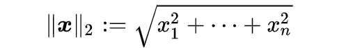
Tuning parameter λ: tuning parameter λ serves to control the relative impact of the penalty on the regression coefficient estimates. When λ = 0, the penalty term has no effect, and the ridge regression will produce the ordinary least squares estimates. But as λ → ∞ (gets very large), the impact of the shrinkage penalty grows, and the ridge regression coefficient estimates approach to 0. Here's a visual representation of this:
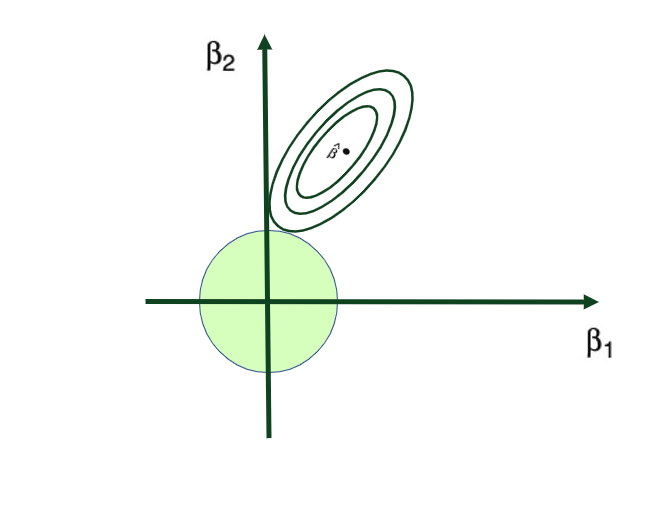
Image Source: The Author
Why does Ridge Regression Work?
Ridge regression’s advantage over ordinary least squares comes from the earlier introduced bias-variance trade-off phenomenon. As λ, the penalty parameter, increases, the flexibility of the ridge regression fit decreases, leading to decreased variance but increased bias.
3.2.2 Lasso Regression (L1 Regularization)
Lasso Regression overcomes this disadvantage of Ridge Regression. Namely, the Lasso Regression coefficient estimates βˆλL are the values that minimize:

As with Ridge Regression, the Lasso shrinks the coefficient estimates towards zero. But in the case of the Lasso, the L1 penalty or L1 norm is used which has the effect of forcing some of the coefficient estimates to be exactly equal to zero when the tuning parameter λ is significantly large.
So, like many feature selection techniques, Lasso Regression performs variable selection besides solving the overfitting problem.
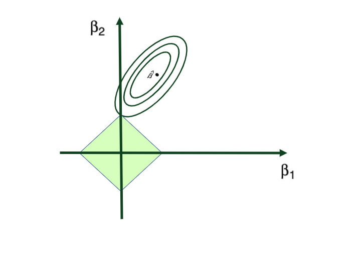
[Image Source: The Author] Lasso regression
L1 Norm (Manhattan Distance)
L1 norm is a mathematical term that comes from Linear Algebra. It stands for a Manhattan norm which can be represented as follows:

Why does Lasso Regression Work?
Like, Ridge Regression, Lasso Regression’s advantage over ordinary least squares comes from the earlier introduced bias-variance trade-off. As λ increases, the flexibility of the ridge regression fit decreases. This leads to decreased variance but increased bias. Additionally, Lasso also performs feature selection.
3.2.3 Lasso vs Ridge Regression
Lasso Regression shrinks the coefficient estimates towards zero and even forces some of these coefficients to be exactly equal to zero when the tuning parameter λ is significantly large. So, like many features selection techniques, Lasso Regression performs variable selection besides solving the overfitting problem.
Comparison between Ridge Regression and Lasso Regression becomes clear when putting earlier two graphs next to each other:
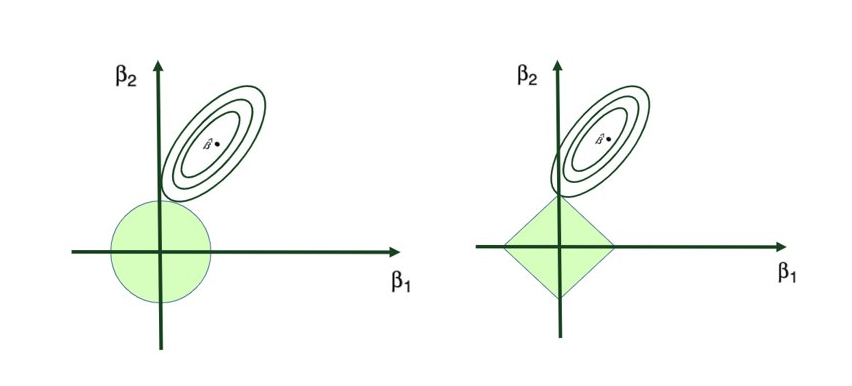
[Image Source: The Author] Lasso regression vs Ridge regression
If you want to learn regularization in detail, read this tutorial:
Chapter 4: Resampling Techniques in Machine Learning
When we have only training data and we want to make judgments about the performance of the model on unseen data, we can use Resampling Techniques to create artificial test data.
Resampling Techniques are often divided into two categories: Cross-Validation and Bootstrapping. They're usually used for the following three purposes:
Model Assessment: evaluate the model performance (to compute test error rate)
Model Variance: compute the variance of the model to check how generalizable your model is
Model Selection: select model flexibility
For example, in order to estimate the variability of a linear regression fit, we can repeatedly draw different samples from the training data, fit a linear regression to each new sample, and then examine the extent to which the resulting fits differ.
4.1 Cross-Validation
Cross-validation can be used to estimate the test error associated with a given statistical learning method in order to perform:
Model assessment: to evaluate its performance by calc test error rate
Model Selection: to select the appropriate level of flexibility.
You hold out a subset of the training observations from the fitting process, and then apply the statistical learning method to those held out observations.
CV is usually divided in the following three categories:
Validation Set Approach
K-fold Cross Validation (K-ford CV)
Leave One Out Cross Validation (LOOCV)
4.1.1 Validation Set Approach
This is a simple approach to randomly split the data into training and validation sets. This approach usually uses Sklearn’s train_test_split() function.
The model is then trained on the training data (usually 80% of the data) and uses it to predict the values for the hold-out or Validation Set (usually 20% of the data) which is the test error rate.
4.1.2 Leave One Out Cross Validation (LOOCV)
LOOCV is similar to the Validation set approach. But each time it leaves one observation out of the training set and uses the remaining n-1 to train the model and calculates the MSE for that one prediction. So, in the case of LOOCV, the Model has to be fit n times (where n is the number of observations in the model).
Then this process is repeated for all observations and n times MSEs are calculated. The mean of the MSEs is the Cross-Validation error rate and can be expressed as follows:

4.1.3 K-fold Cross Validation (K-ford CV)
K-Fold CV is the silver lining between the Validation Set approach (high variance and high bias but is computationally efficient) versus the LOOCV (low bias and low variance but is computationally inefficient).
In K-Fold CV, the data is randomly sampled into K equally sized samples (K- folds). Then each time, 1 is used as validation and the rest as training, and the model is fit K times. The mean of K MSEs form the Cross validation test error rate.
Note that the LOOCV is a special case of K-fold CV where K = N, and can be expressed as follows:

4.2 Selecting Optimal k in K-fold CV
The choice of k in K-fold is a matter of Bias-Variance Trade-Off and the efficiency of the model. Usually, K-Fold CV and LOOCV provide similar results and their performance can be evaluated using simulated data.
However, LOOCV has lower bias (unbiased) compared to K-fold CV because LOOCV uses more training data than K-fold CV does. But LOOCV has higher variance than K-fold does because LOOCV is fitting the model on almost identical data for each item and the outcomes are highly correlated compared to the outcomes of K-Fold which are less correlated.
Since the mean of highly correlated outcomes has higher variance than the one of less correlated outcomes, the LOOCV variance is higher.
K = N (LOOCV) , larger the K→ higher variance and lower bias
K = 1, smaller the K → lower variance and higher bias
Taking this information into account, we can calculate the performance of the model for various Ks lets say K = 3,5,6,7…,10 or the Type I, Type II, and total model classification error in case of classification model. Then the best performing model’s K can be the optimal K using the idea of ROC curve (classification case) or the Elbow method (regression case).
4.3 Bootstrapping
Bootstrapping is another very popular resampling technique that is used for various purposes. One of them is to effectively estimate the variability of the estimates/models or to create artificial samples from an existing sample and improve model performance (like in the case of Bagging or Random Forest).
It is used in many situations where it's hard or even impossible to directly compute the standard deviation of a quantity of interest.
It's a very useful way to quantify the uncertainty associated with the statistical learning method and obtain the standard errors/measure of variability.
It's not useful for Linear Regression since the standard R/Python provides these results (SE of coefficients).
Bootstrapping is extremely handy for other methods as well where variability is more difficult to quantify. The bootstrap sampling is performed with replacement, which means that the same observation can occur more than once in the bootstrap data set.
So, Bootstrapping takes the original training sample and resamples from it by replacement, resulting in B different samples. Then for each of these simulated samples, the coefficient estimate is computed. Then, by taking the mean of these coefficient estimates and using the common formula for SE, we calculate the Standard Error of the Bootstrapped model.
Read more about it here.
Chapter 5: Optimization Techniques
Knowing the fundamentals of the Machine Learning models and learning how to train those models is definitely big part of becoming technical Data Scientist. But that’s only a part of the job.
In order to use the Machine Learning model to solve a business problem, you need to optimize it after you have established its baseline. That is, you need to optimize the set of hyper parameters in your Machine Learning model to find the set of optimal parameters that result in the best performing model (all things being equal).
So, to optimize or to tune your Machine Learning model, you need too perform hyperparameter optimization. By finding the optimal combination of hyper parameter values, we can decrease the errors the model produces and build the most accurate model.
A model hyperparameter is a constant in the model. It's external to the model, and its value cannot be estimated from data (but rather should be specified in advanced before the model is trained). For instance, k in k-Nearest Neighbors (kNN) or the number of hidden layers in Neural Networks.
Hyperparameter optimization methods are usually categorized into:
Exhaustive Search or Brute Force Approach (like Grid Search)
Gradient Descent (Batch GD, SGD, SDG with Momentum, Adam)
Genetic Algorithms
In this handbook, I will discuss only the first two types of optimisation techniques.
5.1 Brute Force Approach (Grid Search)
Exhaustive Search (often referred as Grid Search or Brute Force Approach) is the process of looking for the most optimal hyperparameters by checking each of the candidates for the hyperparameters and computing the model error rate.
Once we create the list of possible values for each of the hyperparameters, for every possible combination of hyper parameter values, we calculate the model error rate and compare it to the current optimal model (one with minimum error rate). During each iteration, the optimal model is updated if the new parameter values result in lower error rate.
The optimisation method is simple. For instance, if you are working with a K-means clustering algorithm, you can manually search for the right number of clusters. But if there are hundreds or thousands of possible combination of hyperparameter values that you have to consider, the model can take hours or days to train – and it becomes incredibly heavy and slow. So most of the time, brute-force search is inefficient.
To optimize or to tune your Machine Learning model, you need to perform hyperparameter optimization. By finding the optimal combination of hyper parameter values, we can decrease the error the model produces and build the most accurate model.
When it comes to Gradient Descent type of optimisation techniques, then its variants such as Batch Gradient Descent, Stochastic Gradient Descent, and so on differ in terms of the amount of data used to compute the gradient of the Loss or Cost function.
Let's define this Loss Function by J(θ) where θ (theta) represents the parameter we want to optimize.
The amount of data usage is about a trade-off between the accuracy of the parameter update and the time it takes to perform such an update. Namely, the larger the data sample we use, we can expect a more accurate adjustment of a parameter – but the process will be then much slower.
The opposite holds true as well. The smaller the data sample, the less accurate will be the adjustments in the parameter but the process will be much faster.
5.2 Gradient Descent Optimization (GD)
The Batch Gradient Descent algorithm (often just referred to as Gradient Descent or GD), computes the gradient of the Loss Function J(θ) with respect to the target parameter using the entire training data.
We do this by first predicting the values for all observations in each iteration, and comparing them to the given value in the training data. These two values are used to calculate the prediction error term per observation which is then used to update the model parameters. This process continues until the model converges.
The gradient or the first order derivative of the loss function can be expressed as follows:

Then, this gradient is used to update the previous iterations’ value of the target parameter. That is:

where
θ: This represents the parameter(s) or weight(s) of a model that you are trying to optimize. In many contexts, especially in neural networks, θ can be a vector containing many individual weights.
η: This is the learning rate. It's a hyperparameter that dictates the step size at each iteration while moving towards a minimum of the cost function. A smaller learning rate might make the optimization more precise but could also slow down the convergence process, while a larger learning rate might speed up convergence but risks overshooting the minimum. Can be [0,1] but is is usually a number between (0.001 and 0.04)
∇_J_(θ): This is the gradient of the cost function J with respect to the parameter θ It indicates the direction and magnitude of the steepest increase of J. By subtracting this from the current parameter value (multiplied by the learning rate), we adjust θ in the direction of the steepest decrease of J.
There are two major disadvantages to GD which make this optimization technique not so popular especially when dealing with large and complex datasets. Since in each iteration the entire training data should be used and stored, the computation time can be very large resulting in incredibly slow process. On top of that, storing that large amount of data results in memory issues, making GD computationally heavy and slow.
5.3 Stochastic Gradient Descent (SGD)
The Stochastic Gradient Descent (SGD) method, also known as Incremental Gradient Descent, is an iterative approach for solving optimisation problems with a differential objective function, exactly like GD.
But unlike GD, SGD doesn’t use the entire batch of training data to update the parameter value in each iteration. The SGD method is often referred as the stochastic approximation of the gradient descent which aims to find the extreme or zero points of the stochastic model containing parameters that cannot be directly estimated.
SGD minimises this cost function by sweeping through data in the training dataset and updating the values of the parameters in every iteration.
In SGD, all model parameters are improved in each iteration step with only one training sample. So, instead of going through all training samples at once to modify model parameters, the SGD algorithm improves parameters by looking at a single and randomly sampled training set (hence the name Stochastic). That is:

where
θ: This represents the parameter(s) or weight(s) of a model that you are trying to optimize. In many contexts, especially in neural networks, θ can be a vector containing many individual weights.
η: This is the learning rate. It's a hyperparameter that dictates the step size at each iteration while moving towards a minimum of the cost function. A smaller learning rate might make the optimization more precise but could also slow down the convergence process, while a larger learning rate might speed up convergence but risks overshooting the minimum.
∇_J_(θ,x(i),y(i)): This is the gradient of the cost function J with respect to the parameter θ for a given input x(i) and its corresponding target output y(i). It indicates the direction and magnitude of the steepest increase of J. By subtracting this from the current parameter value (multiplied by the learning rate), we adjust θ in the direction of the steepest decrease of J.
x(i): This represents the ith input data sample from your dataset.
y(i): This is the true target output for the ith input data sample.
In the context of Stochastic Gradient Descent (SGD), the update rule applies to individual data samples x(i) and y(i) rather than the entire dataset, which would be the case for batch Gradient Descent.
This single-step improves the speed of the process of finding the global minima of the optimization problem and this is what differentiate SGD from GD. So, SGD consistently adjusts the parameters with an attempt to move in the direction of the global minimum of the objective function.
SGD addresses the slow computation time issue of GD, because it scales well with both big data and with a size of the model. But even though SGD method itself is simple and fast, it is known as a “bad optimizer” because it's prone to finding a local optimum instead of a global optimum.
In SGD, all model parameters are improved in each iteration step with only one training sample. So, instead of going through all training samples at once to modify model parameters, SGD improves parameters by looking at a single training sample.
This single step improves the speed of the process of finding the global minimum of the optimization problem. This is what differentiates SGD from GD.
5.4 SGD with Momentum
When the error function is complex and non-convex, instead of finding the global optimum, the SGD algorithm mistakenly moves in the direction of numerous local minima. This results in higher computation time.
In order to address this issue and further improve the SGD algorithm, various methods have been introduced. One popular way of escaping a local minimum and moving right in direction of a global minimum is SGD with Momentum.
The goal of the SGD method with momentum is to accelerate gradient vectors in the direction of the global minimum, resulting in faster convergence.
The idea behind the momentum is that the model parameters are learned by using the directions and values of previous parameter adjustments. Also, the adjustment values are calculated in such a way that more recent adjustments are weighted heavier (they get larger weights) compared to the very early adjustments (they get smaller weights).
The reason for this difference is that with the SGD method we do not determine the exact derivative of the loss function, but we estimate it on a small batch. Since the gradient is noisy, it is likely that it will not always move in the optimal direction.
The momentum helps then to estimate those derivatives more accurately, resulting in better direction choices when moving towards the global minimum.
Another reason for the difference in the performance of classical SGD and SGD with momentum lies in the area referred as Pathological Curvature, also called the ravine area.
Pathological Curvature or Ravine Area can be represented by the following graph. The orange line represents the path taken by the method based on the gradient while the dark blue line represents the ideal path in towards the direction of ending the global optimum.
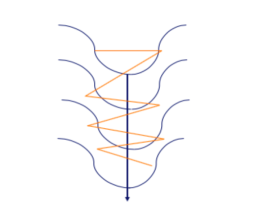
Image Source: The author
To visualise the difference between the SGD and SGD Momentum, let's look at the following figure.

Image Source: The author
In the left hand-side is the SGD method without Momentum. In the right hand-side is the SGD with Momentum. The orange pattern represents the path of the gradient in a search of the global minimum.
The idea behind the momentum is that the model parameters are learned by using the directions and values of previous parameter adjustments. Also, the adjustment values are calculated in such a way that more recent adjustments are weighted heavier (they get larger weights) compared to the very early adjustments (they get smaller weights).
5.5 Adam Optimizer
Another popular technique for enhancing SGD optimization procedure is the Adaptive Moment Estimation (Adam) introduced by Kingma and Ba (2015). Adam is the extended version of the SGD with the momentum method.
The main difference compared to the SGD with momentum, which uses a single learning rate for all parameter updates, is that the Adam algorithm defines different learning rates for different parameters.
The algorithm calculates the individual adaptive learning rates for each parameter based on the estimates of the first two moments of the gradients (first and the second order derivative of the Loss function).
So, each parameter has a unique learning rate, which is being updated using the exponential decaying average of the rst moments (the mean) and second moments (the variance) of the gradients.
Key Takeaways & What Comes Next
In this handbook, we've covered the essentials and beyond in machine learning. From the basics to advanced techniques, we've unpacked popular ML algorithms used globally in tech and the key optimization methods that power them.
While learning about each concept, we saw some practical examples and Python code, ensuring that you're not just understanding the theory but also its application.
Your Machine Learning journey is ongoing, and this guide is your reference. It's not a one-time read – it's a resource to revisit as you progress and flourish in this field. With this knowledge, you're ready to tackle most of the real-world ML challenges confidently at a high level. But this is just the beginning.
About the Author — That’s Me!
I am Tatev, Senior Machine Learning and AI Researcher. I have had the privilege of working in Data Science across numerous countries, including the US, UK, Canada, and the Netherlands.
With an MSc and BSc in Econometrics under my belt, my journey in Machine and AI has been nothing short of incredible. Drawing from my technical studies during my Bachelors & Masters, along with over 5 years of hands-on experience in the Data Science Industry, in Machine Learning and AI, I've gathered this high-level summary of ML topics to share with you.
How Can You Dive Deeper?
After studying this guide, if you're keen to dive even deeper and structured learning is your style, consider joining us at LunarTech. Follow the course "Fundamentals to Machine Learning," a comprehensive program that offers an in-depth understanding of the theory, hands-on practical implementation, extensive practice material, and tailored interview preparation to set you up for success at your own phase.
This course is also a part of The Ultimate Data Science Bootcamp which has earned the recognition of being one of the Best Data Science Bootcamps of 2023, and has been featured in esteemed publications like Forbes, Yahoo, Entrepreneur and more. This is your chance to be a part of a community that thrives on innovation and knowledge. You can enroll for a Free Trial of The Ultimate Data Science Bootcamp at LunarTech.
Connect with Me:

Image Source: LunarTech
Follow me on LinkedIn for a ton of Free Resources in ML and AI
Subscribe to my The Data Science and AI Newsletter
Want to discover everything about a career in Data Science, Machine Learning and AI, and learn how to secure a Data Science job? Download this FREE Data Science and AI Career Handbook
Thank you for choosing this guide as your learning companion. As you continue to explore the vast field of machine learning, I hope you do so with confidence, precision, and an innovative spirit. Best wishes in all your future endeavors!