

When you're working in Excel, the VLOOKUP function makes looking up information less time-consuming. This is particularly true when you're using more than one Excel sheet.
In this article, you will learn what the VLOOKUP function does, as well as understand the syntax behind it. You will also learn how to use the VLOOKUP Excel function to search for a value with the help of a simple example.
Let's get started!
What Is VLOOKUP in Excel? VLOOKUP Definition
VLOOKUP is a powerful Microsoft Excel function that searches for and retrieves information from a table of data.
VLOOKUP stands for Vertical Lookup, so the V in VLOOKUP is short for Vertical.
Vertical in Excel refers to columns and, in this case, looking up data vertically across the spreadsheet.
Specifically, VLOOKUP looks for a specific value in a column.
VLOOKUP looks up a specific piece of information in a dataset and returns additional data related to that initial information but from a different column in the same row.
For example, if you have a list of names and emails, VLOOKUP will look up a person's name in a table and retrieve their email. This will be the email entry associated with their name.
Something to note is that VLOOKUP should not be confused with HLOOKUP - HLOOKUP is an entirely different function.
HLOOKUP stands for Horizontal Lookup, and the H is short for Horizontal. Horizontal in Excel refers to rows and searching for data horizontally across the spreadsheet.
To learn more about rows and columns in Excel, read this quick quide that explains the difference between the two.
VLOOKUP Function Syntax Breakdown
The general syntax for the VLOOKUP function is the following:
=VLOOKUP(lookup_value, table_array, column_number, [range_lookup])
You start by writing an equals sign, =, and then you type the VLOOKUP() function.
The VLOOKUP function takes four arguments, and each argument is separated by a comma, ,.
Let's explain what each argument means:
- lookup_value: This argument is required and specifies the value you want to look up and locate. This value is at the leftmost corner and in the first column of the table. VLOOKUP will always search for information to the right of this
lookup_value. - table_array: This argument is required and represents the range of data in the table that you want to search through. The
lookup_value, thecolumn_number, and the return value you want to get are all included in this range. - column_number: This argument is required. It is an integer number that specifies the column number in the
table_arrayfrom which you want to retrieve the return value. - range_lookup: This argument is optional and is either
TRUEorFALSE.TRUEspecifies that the function should return an approximate match, meaning that if there is no exact match, it should return the closest match possible. AndFALSEspecifies that the function should return an exact match for what you are looking for, and if it doesn't, this will result in an error.
How to Use VLOOKUP in Excel
Below I have an example of a simple dataset.
This example will give you an idea of how you can use the VLOOKUP function. You can also apply the techniques used here to larger and more complex tables.
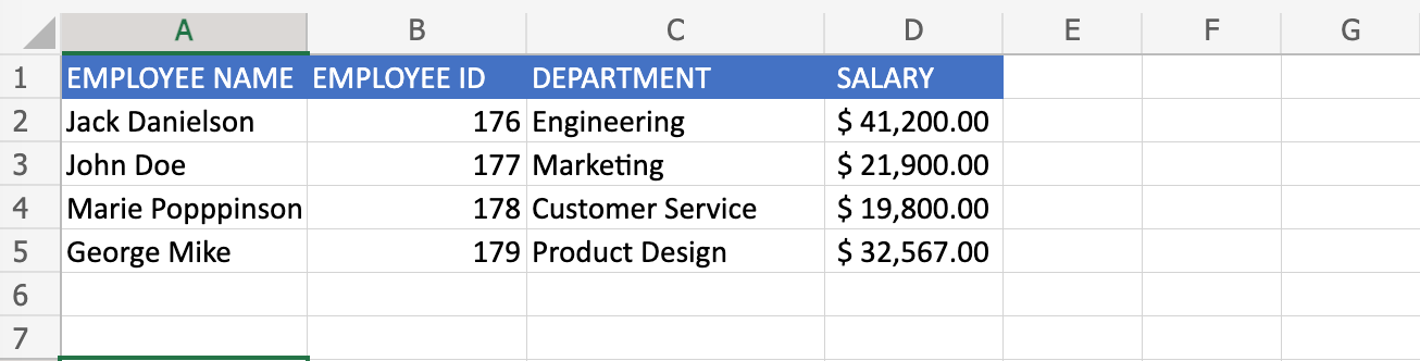
I am going to use VLOOKUP to search through a table of employee data. This table stores an employee's name, id number, the department they work in, and their salary.
I want to use VLOOKUP to search for a specific employee and have their matching salary returned.
I want it so that whenever I search for an employee's name in the F2 cell, their corresponding salary is returned.
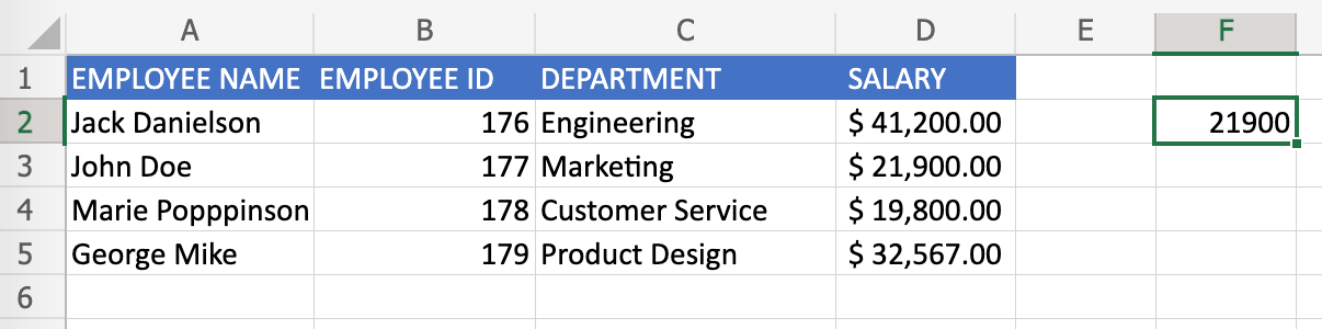
So, If I wanted to locate the employee John Doe and return their salary, in column F2, I would write:
=VLOOKUP(A3, A2:D5, 4, FALSE)
Let's break it down:
- The cell
A3contains the value that I want to search for. The employee namedJohn Doeis located in cellA3. This will be the lookup value and the first argument of the function. - The range of cells
A2:D5contains the data I want to search through. This is the source of data VLOOKUP will use. This range needs to include the first column, which stores the first argument, and it also needs to include the column where I hope the return value is stored. - Next, I include the column number where the return value can be found. Keep in mind that you need to start counting where the table begins. In this case, it is the
4th column in the table. - Lastly, I want VLOOKUP to return an exact match, so the last argument is
FALSE.
I then see the result in the F2 cell:
Conclusion
In this article, you learned the basics of using the VLOOKUP function in Excel.
To learn more about Excel, check out the following resources:
Thanks for reading!