By Vardan Grigoryan (vardanator)
Graph theory represents one of the most important and interesting areas in computer science. But at the same time it’s one of the most misunderstood (at least it was to me).
Understanding, using and thinking in graphs makes us better programmers. At least that’s how we’re supposed to think. A graph is a set of vertices V and a set of edges E, comprising an ordered pair G=(V, E).
While trying to studying graph theory and implementing some algorithms, I was regularly getting stuck, just because it was so boring.
The best way to understand something is to understand its applications. In this article, we’re going to demonstrate various applications of graph theory. But more importantly, these applications will contain detailed illustrations. So lets get started and dive in.
While this approach might seem too detailed (to seasoned programmers), but believe me, as someone who was once there and tried to understand graph theory, detailed explanations are always preferred over succinct definitions.
So, if you’ve been looking for a “graph theory and everything about it tutorial for absolute unbelievable dummies”, then you’ve come to the right place. Or at least I hope. So lets get started and dive in.
 He meant Monte Cristo
Table of Contents
- Disclaimers
- Seven Bridges of Königsberg
- Graph representation: Intro
- Intro to Graph representation and binary trees (Airbnb example)
- Graph representation: Outro
- Twitter example: tweet delivery problem
- Graph Algorithms: intro
- Netflix and Amazon: inverted index example
- Traversals: DFS and BFS
- Uber and the shortest path problem (Dijkstra’s algorithm)
Disclaimers
DISCLAIMER 1: I am not an expert in CS, algorithms, data structures and especially in graph theory. I am not involved in any project for the companies discussed in this article. Solutions to the problems are not final and could be improved drastically. If you find any issue or something unreasonable, you are more than welcome to leave a comment. If you work at one of the mentioned companies or are involved in corresponding software projects, please respond with the actual solution (it will be helpful to others). To all others, be patient readers, this is a pretty LONG article.
DISCLAIMER 2: This article is somewhat different in the style that information is provided. Sometimes it might seem a bit digressed from the sub-topic, but patient readers will eventually find themselves with a complete understanding of the bigger picture.
DISCLAIMER 3: This article is written for a broad audience of programmers. While having junior programmers as the target audience, I hope it will be interesting to experienced professionals as well.
Seven Bridges of Königsberg
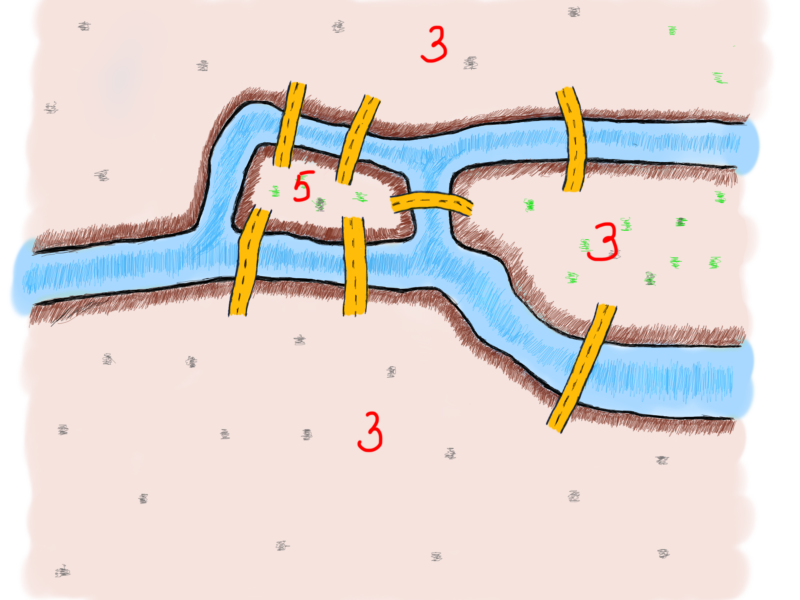
Let’s start with something that I used to regularly encounter in graph theory books that discuss “the origins of graph theory”, the Seven Bridges of Königsberg (not really sure, but you can pronounce it as “qyonigsberg”). There were seven bridges in Kaliningrad, connecting two big islands surrounded by the Pregolya river and two portions of mainlands divided by the same river.
 _[Our area of interest](https://www.google.com.au/maps/@54.7066964,20.5100082,16z" rel="noopener" target="blank" title=")
In the 18th century this was called Königsberg (part of Prussia) and the area above had a lot more bridges. The problem or just a brain teaser with Königsberg’s bridges was to be able to walk through the city by crossing all the seven bridges only once. They didn’t have an internet connection at that time, so it should have been entertaining. Here’s the illustrated view of the seven bridges of Königsberg in 18th century.
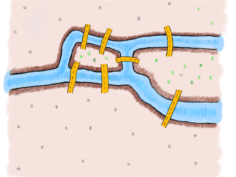 Seven bridges of Königsberg
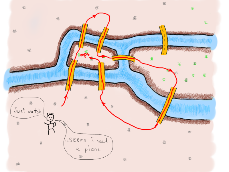
Try it. See if you can walk through the city by crossing each bridge only once.
- There should not be any uncrossed bridge(s).
- Each bridge must not be crossed more than once.
If you are familiar with this problem, you know that it’s impossible to do it. Although you were trying hard enough and you may try even harder now, you’ll eventually give up.
 Leonhard Euler (photo from Wikipedia)
Sometimes it’s reasonable to give up fast. That’s how Euler solved this problem - he gave up pretty soon. Instead of trying to solve it, he adopted a different approach of trying to prove that it’s not possible to walk through the city by crossing each bridge one and only time.
Let’s try to understand how Euler was thinking and how he came up with the solution (if there isn’t a solution, it still needs a proof). That is a real challenge here, because walking through the thought process of such a venerable mathematician is kind of dishonorable. (Venerable so much that Knuth and friends dedicated their book to Leonhard Euler). We rather will pretend to “think like Euler”. Let’s start with picturing the impossible.
There are four distinct places, two islands and two parts of mainland. And seven bridges. It’s interesting to find out if there is any pattern regarding the number of bridges connected to islands or mainland (we will use the term “land” to refer to the four distinct places).
 Number of bridges
At a first glance, there seems to be some sort of a pattern. There are an odd number of bridges connected to each land. If you have to cross each bridge once, then you can enter a land and leave it if it has 2 bridges.
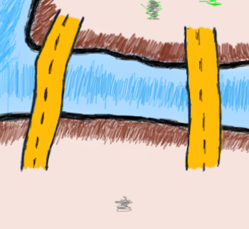
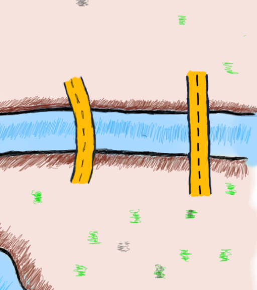 Examples of 2 bridge lands
It’s easy to see in the illustrations above that if you enter a land by crossing one bridge, you can always leave the land by crossing its second bridge. Whenever a third bridge appears, you won’t be able to leave a land once you enter it by crossing all its bridges. If you try to generalize this reasoning for a single piece of land, you’ll be able to show that, in case of an even number of bridges it’s always possible to leave the land and in case of an odd number of bridges it isn’t. Try it in your mind!
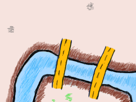
Let’s add a new bridge to see how the number of overall connected bridges changes and whether it solves the problem.
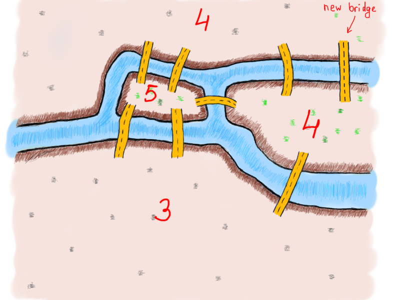 Notice the new bridge
Now that we have two even (4 and 4) and two odd (3 and 5) number of bridges connecting the four pieces of land, let’s draw a new route with the addition of this new bridge.
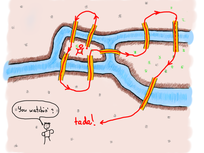 Wow
Wow
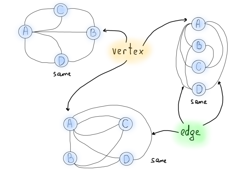
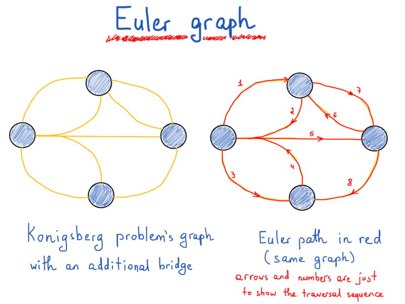
We saw that the number of even and odd number of bridges played a role in determining if the solution was possible. Here’s a question. Does the number of bridges solve the problem? Should it be even all the time? Turns out that it’s not the case. That’s what Euler did. He found a way to show that the number of bridges matter. And more interestingly, the number of pieces of land with an odd number of connected bridges also matters. That’s when Euler started to “convert” lands and bridges into something we know as graphs. Here’s how a graph representing the Königsberg bridges problem could look like (note that our “temporarily” added bridge isn’t there).
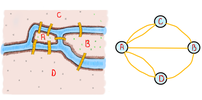 Lines are a bit twisty
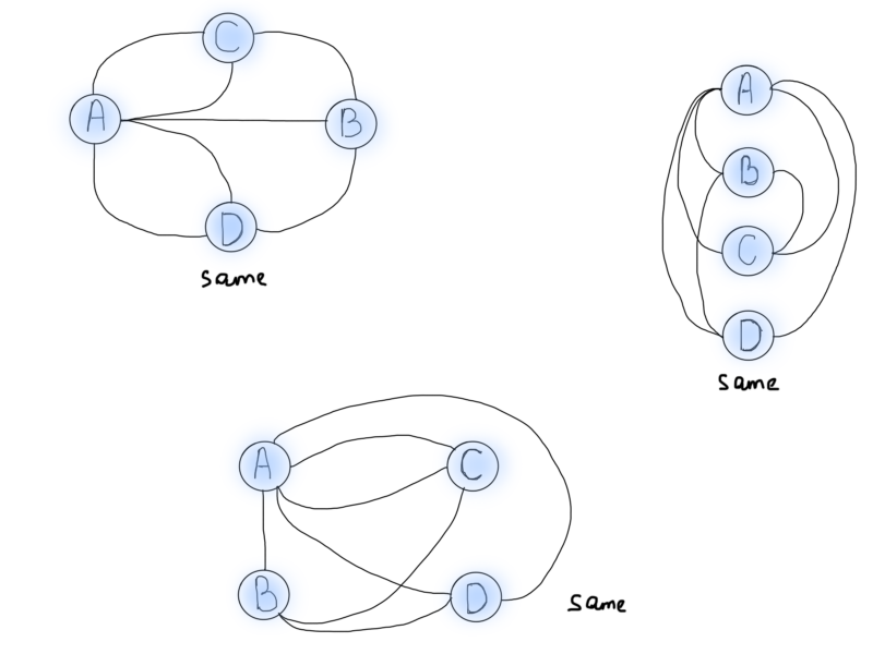
One important thing to note is the generalization/abstraction of a problem. Whenever you solve a specific problem, the most important thing is to generalize the solution for similar problems. In this particular case, Euler’s task was to generalize the bridge crossing problem to be able to solve similar problems in the future, i.e. for all the bridges in the world. Visualization also helps to view the problem at a different angle. The following graphs are all various representations of the same Königsberg bridge problem shown above.
So yes, visually graphs are a good choice for picturing problems. But now we need to find out how the Königsberg problem can be solved using graphs. Pay attention to the number of lines coming out of each circle. And yes, let’s name them as seasoned professionals would do, from now on we will call circles, vertices and the lines connecting them, edges. You might’ve seen letter notations, V for (vendetta?) vertex, E for edge.
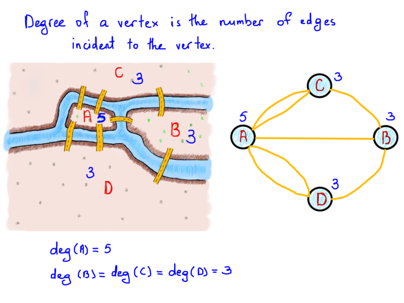
The next important thing is the so-called degree of a vertex, the number of edges incident connected to the vertex. In our example above, the number of bridges connected to lands can be expressed as degrees of the graph vertex.
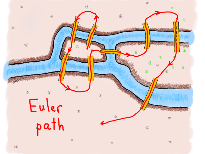
In his endeavor Euler showed that the possibility of a walk through graph (city) traversing each edge (bridge) one and only one time is strictly dependent on the degrees of vertices (lands). The path consisting of such edges called (in his honor) an Euler path. The length of an Euler path is the number of edges. Get ready for some strict language. ?
An Euler path of a finite undirected graph G(V, E) is a path such that every edge of G appears on it once. If G has an Euler path, then it is called an Euler graph. [1]
Theorem. A finite undirected connected graph is an Euler graph if and only if exactly two vertices are of odd degree or all vertices are of even degree. In the latter case, every Euler path of the graph is a circuit, and in the former case, none is. [1]
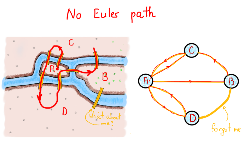 Exactly two vertices have an odd degree in the illustration at the left, and all vertices are of an odd degree in illustration at the right
I used “Euler path” instead of “Eulerian path” just to be consistent with the referenced books [1] definition. If you know someone who differentiates Euler path and Eulerian path, and Euler graph and Eulerian graph, let them know to leave a comment.
First of all, let’s clarify the new terms in the above definition and theorem.
- Undirected graph - a graph that doesn’t have a particular direction for edges.
- Directed graph - a graph in which edges have a particular direction.
- Connected graph - a graph where there is no unreachable vertex. There must be a path between every pair of vertices.
- Disconnected graph - a graph where there are unreachable vertices. There is not a path between every pair of vertices.
- Finite graph - a graph with a finite number of nodes and edges.
- Infinite graph - a graph where an end of the graph in a particular direction(s) extends to infinity.
We’ll discuss some of these terms in the coming paragraphs.
Graphs can be directed and undirected, and that’s one of the interesting properties of graphs. You must’ve seen a popular Facebook vs Twitter example for directed and undirected graphs. A Facebook friendship relation may be easily represented as an undirected graph, because if Alice is a friend with Bob, then Bob must be a friend with Alice, too. There is no direction, both are friends with each other.
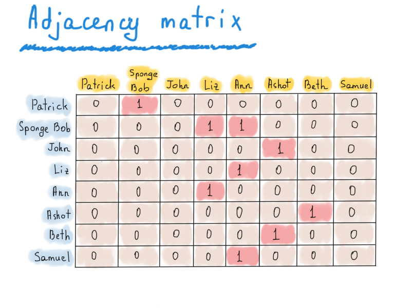
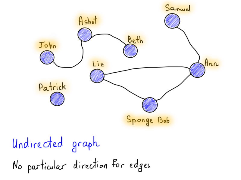 Undirected Graph
Also note the vertex labeled as “Patrick”, it is kind of special (he’s got no friends), as it doesn’t have any incident edges. It is still a part of the graph, but in this case we will say that this graph is not connected, it is a disconnected graph (same goes with “John”, “Ashot” and “Beth” as they are interconnected with each other but separated from others). In a connected graph there is no unreachable vertex, there must be a path between every pair of vertices.
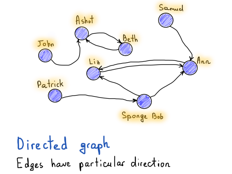
Contrary to the Facebook example, if Alice follows Bob on Twitter, that doesn’t require Bob to follow Alice back. So a “follow” relation must have a direction indicator, showing which vertex (user) has a directed edge (follows) to the other vertex.
Now, knowing what is a finite connected undirected graph, let’s get back to Euler’s graph:
So why did we discuss Königsberg bridges problem and Euler graphs in the first place? Well, it’s not so boring and by investigating the problem and foregoing solution we touched the elements behind graphs (vertex, edge, directed, undirected) avoiding a dry theoretical approach. And no, we are not done with Euler graphs and the problem above, yet. ?
We should now move on to the computer representation of graphs as that is the topic of interest for us programmers. By representing a graph in a computer program, we will be able to devise an algorithm for tracing graph path(s), and therefore find out if it is an Euler path. Before that, try to think of a good application for an Euler graph (besides fiddling around with bridges).
Graph representation: Intro
Now this is quite a tedious task, so be patient. Remember the fight between Arrays and Linked Lists? Use arrays if you need fast element access, use lists if you need fast element insertion/deletion, etc. I hardly believe you ever struggled with something like “how to represent lists”. Well, in case of graphs the actual representation is really bothering, because first you should decide how exactly are you going to represent a graph. And believe me, you are not going to like this. Adjacency list, adjacency matrix, maybe edge lists? Toss a coin.
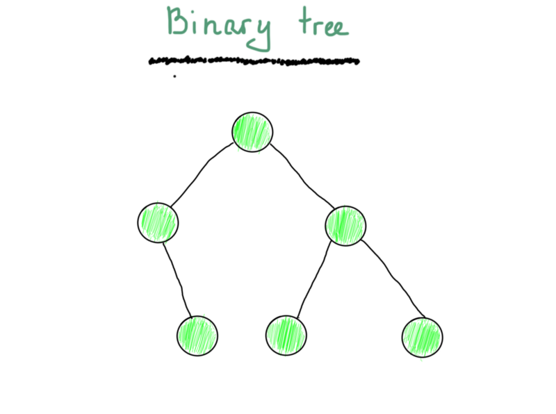
You should have tossed hard, because we are starting with a tree. You must have seen a binary tree (or BT for short) at least once (the following is not a binary search tree).
 Just a sample
Just because it consists of vertices and edges, it’s a graph. You also may recall how most commonly a binary tree is represented (at least in textbooks).
It might seem too basic for people who are already familiar with binary trees, but I still have to illustrate it to make sure we are on the same page (note that we are still dealing with pseudocode).
If you are new to trees, read the pseudocode above carefully, then follow the steps in the illustration below.
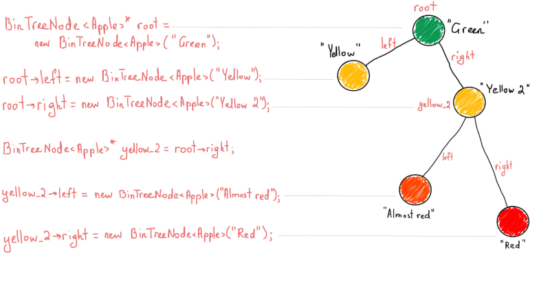 Colors are just for bright visualization
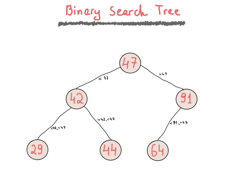
While a binary tree is a simple “collection” of nodes, each of which has left and right child nodes. A binary search tree is much more useful as it applies one simple rule which allows fast key lookups. Binary search trees (BST) keep their keys in sorted order. You are free to implement your BT with any rule you want (although it might change its name based on the rule, for instance, min-heap or max-heap). The most important expectation for a BST is that it satisfies the binary search property (that’s where the name comes from). Each node’s key must be greater than any key in its left sub-tree and less than any key in its right sub-tree.
I’d like to point out a very interesting point regarding the statement “greater than” that’s crucial to understand how BST’s function. Whenever you change the property to “greater than or equal”, your BST will be able to save duplicate keys when inserting new nodes, otherwise it will keep only nodes with unique keys. You can find really good articles on the web about binary search trees. We won’t be providing a full implementation of a binary search tree, but for the sake of consistency, we’ll illustrate a simple binary search tree here.
Intro to Graph representation and binary trees (Airbnb example)
Trees are very useful data structures. You might not have implemented a tree from scratch in your projects. But you’ve probably used them even without noticing. Let’s look at an artificial yet valuable example and try to answer the “why” question, “Why use a binary search tree in the first place”.
As you’ve noticed, there is a “search” in binary search tree. So basically, everything that needs a fast lookup, should be placed in a binary search tree. “Should” doesn’t mean must, the most important thing to keep in mind in programming is to solve a problem with proper tools. There are tons of cases where a simple linked list with its O(N) lookup might be more preferable than a BST with its O(logN) lookup.
Typically we would use a library implementation of a BST, most likely std::set or std::map in C++. However in this tutorial we are free to reinvent our own wheel. BSTs are implemented in almost any general-purpose programming language library. You can find them in the corresponding documentation of your favorite language. Approaching a “real-life example”, here’s the problem we’ll try to tackle - Airbnb Home Search.
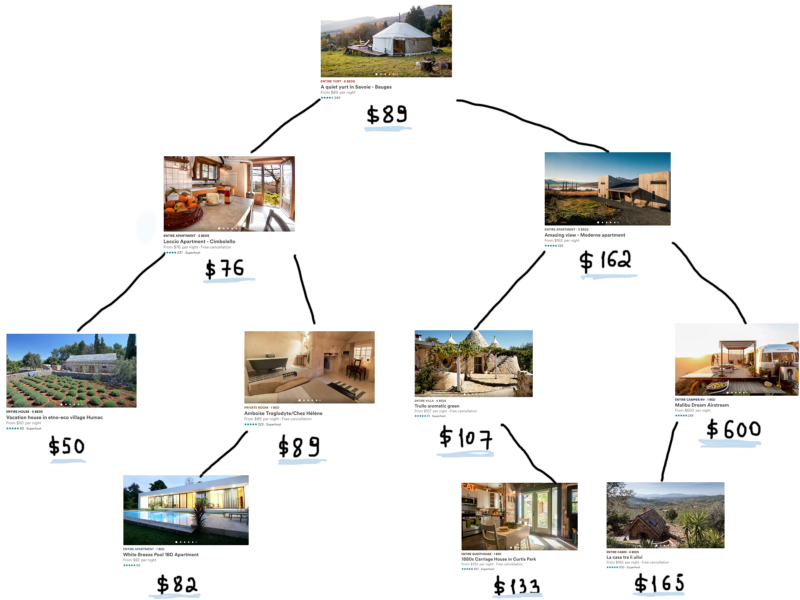
 A glimpse on Airbnb Homes Search
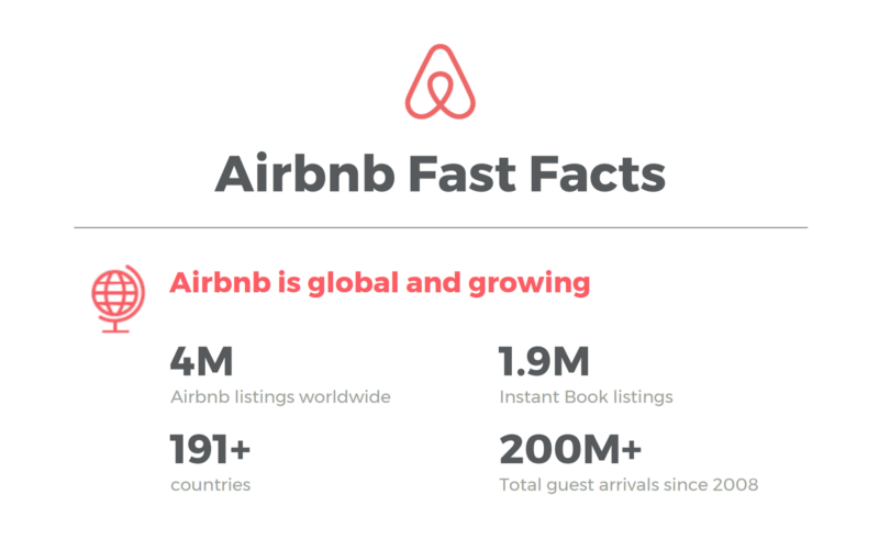
How do we search for homes based on some query with a bunch of filters as fast as possible. This is a hard task. It becomes harder if we consider that Airbnb stores 4 millions listings.
So when users search for homes, there is a chance that they might “touch” 4 million records stored in the database. Sure the results are limited to the “top listings” shown on the website’s home page and a user almost is never curious “enough” to view millions of listings. I don’t have any analytics regarding Airbnb, but we can use a powerful tool in programming called “assumptions”. So we will assume that a single user finds a good home by viewing at most ~1K homes.
The most important factor here is the number of real-time users, as it makes a difference in data structures and database(s) choices and the project architecture overall. As obvious as it might seem, if there are just 100 users overall, then we may not bother at all.
On the contrary, if the number of users overall and real-time users in particular is far beyond the million threshold, we have to think really wisely about each decision. “Each” is used exactly right, that’s why companies hire the best while striving for excellence in service provision.
Google, Facebook, Airbnb, Netflix, Amazon, Twitter, and many others deal with huge amounts of data and the right choice to serve millions of bytes of data each second to millions of real-time users starts from hiring the right engineers. That’s why we, the programmers, struggle with these data structures, algorithms and problem solving in possible interviews, because all they need is the engineer having the ability to solve such big problems in the fastest and most efficient possible way.
So here’s a use case. A user visits the home page (we’re still talking about Airbnb) and tries to filter out homes to find the best possible fit. How would we deal with this problem? (Note that this problem is rather backend-side, so we won’t care about front-end or the network traffic or https over http or Amazon EC2 over home cluster and so on).
First of all, as we are already familiar with one of the most powerful tools in a programmers’ inventory (talking about assumptions rather than abstractions), let’s start with a few assumptions:
- We’re dealing with data that completely fits in the RAM.
- Our RAM is big enough.
Big enough to hold, hmm, how much? Well that’s a good question. How much memory will be required to store the actual data. If we are dealing with 4 million units of data (again, am assumption), and if we probably know each unit’s size, then we can easily derive the required memory size, i.e. 4M * sizeof(one_unit).
Let’s consider a “home” object and its properties. Actually, let’s consider at least those properties that we will deal with while solving our problem (a “home” is our unit). We will represent it as a C++ structure in some pseudocode. You can easily convert it to a MongoDB schema object or anything you want. We just discuss the property names and types (try to think about using bitfields or bitsets for space economy).
The above structure is not perfect (obviously) and there are many assumptions and/or incomplete parts. I just looked at Airbnb’s filters and devised property lists that should exist to satisfy search queries. It’s just an example.
Now we should calculate how many bytes in memory will take each AirbnbHome object.
- Home name -
nameis awstringto support multilingual names/titles, which means each character will take 2 bytes (we may not bother with character size if we would use other language, but in C++charis 1-byte character andwcharis 2-byte character). A quick look at Airbnb’s listings allows us to assume that the name of a home should take up to 100 characters (though mostly it is around 50, rather than 100), we’ll assume 100 characters as a maximum value, which leads to ~200 bytes of memory.uintis 4 bytes,ucharis 1 byte,ushortis 2 bytes (again, in our assumptions). - Photos - Photos are residing within some storage service, like Amazon S3 (as far as I know, this assumption is most likely to be true for Airbnb, but again, Amazon S3 is just an assumption)
- Photo URLs - We have those photo URLs, and considering the fact that there is no standard size limit on the URLs, but there is in fact a well-known limit of 2083 characters, we‘ll take it as a max size of any URL. So taking into account that each home has 5 photos in average, it would take up to ~10Kb.
- Photo IDs - Let’s have a rethink about this. Usually storage services serve content with the same base URLs, like
http(s)://s3.amazonaws.com/<bucket>/<object>, i.e. there is a common pattern for constructing URLs and we need to store only the actual photo ID. Let’s say we use some unique ID generator, which returns a 20 byte unique string ID where photo objects and the URL pattern for particular photolooks like https://s3.amazonaws.com/some-know-bucket/<unique-photo-id>. This gives us good space efficiency, so for storing string IDs of five photos we will need only 100 bytes of memory. - Host ID - The same “trick” (above) could be done with the
host_id, i.e. the user ID who hosts the home, takes 20 bytes of memory (actually we could just use integer IDs for users, but considering that some DB systems like MongoDB have rather specific unique ID generator, we’re assuming a 20 byte length string ID as some “median” value which fits into almost any DB system with a little change. Mongo’s ID length is 24 bytes). And finally, we’ll take a bitset of up to 32 bits in size as a 4 bytes object and a bitset of size between 32 and 64 bits, as a 8 byte object. Mind the assumptions. We used bitset in this example for any property that expresses an enum, but is able to take more than one value, in other words a kind of multiple choice checkbox.
 Airbnb House Amenities
Amenities - Each Airbnb home keeps a list of available amenities, e.g. “iron”, “washer”, “tv”, “wifi”, “hangers”, “smoke detector” and even “laptop friendly workspace” and so on. There might be more than 20 amenities, we stick to the 20 just because it’s the number of filterable amenities on the Airbnb filters page. Bitset saves us some good space, if we keep proper ordering for amenities. For instance, if a home has all above mentioned amenities (see checked ones in the screenshot), we will just set a bit at corresponding position in the bitset.
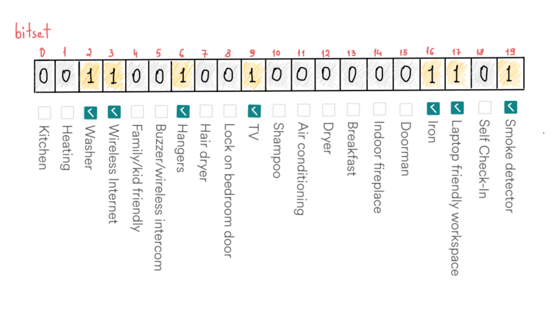 Bitset allows to save 20 different values using just 20 bits
For example, checking if a home has a “washer”:
Or a little more professionally:
You can improve the code as much as you want (and fix compile errors). We just wanted to emphasize the idea behind bitsets in this problem context.
- House rules, Home Type - The same idea (that we implemented for the amenities field) goes with “house rules”, “home type” and others.
- Country code, City name - Finally, the country code and city name. As mentioned in the comments of the code above (see remarks), we won’t store latitude and longitude to avoid geo-spatial queries (a subject of another article). Instead, we save country code and city name to narrow down the search by a location (omitting streets for the sake of simplicity, please forgive me). Country code could be represented as 2 characters, 3 characters or 3 digits, we’ll save a numeric representation and will use an
ushortfor it. (Un)fortunately there are many more cities than countries, so we can’t use a “city code” (though we can make one for internal use). Instead we’ll store actual city name, preserving 50 bytes in average for a city name and for super-specific cases like Taumatawhakatangihangakoauauotamateaturipukakapikimaungahoronukupokaiwhenuakitanatahu (85 letter city). We better use an additional boolean variable which indicates that this is that specific super-long city (don’t try to pronounce it). So, keeping in mind the memory overhead of strings and vectors. We’ll add an additional 32 bytes (just in case) to the final size of the struct. We also will assume that we work on a 64-bit system, although we chose very compact values forintandshort.
So, 420+ bytes with an overhead of 32 bytes, 452 bytes and considering the fact that some of you might just be obsessed with the aligning factor, let’s round up it to 500 bytes. So each “home” object takes up to 500 bytes, and for all home listings (there could be some confusing moments with the listings count and actual home count, just let me know if I got something wrong), 500 bytes 4 million = 1.86GB ~ *2GB. Seems plausible. We made many assumptions while constructing the struct, making it cheaper to save in memory, I really expected much more than 2 Gigabytes and if I did a mistake in calculations, let me know. Anyway, moving forward, so whatever we gonna do with this data, we will need at least 2 GB of memory. If you got bored, deal with it. We are just starting.
Now the hardest part of the task. Choosing the right data structure for this problem (filter the listings as efficiently as possible) is not the hardest task. The hardest task is (for me) to search listings by a bunch of filters. If there would be just one search key (just one filter) we would easily solve it. Suppose the only thing users care is the price, so all we need is to find AirbnbHome objects with prices falling in the provided range. If we’ll use a binary search tree for that, here’s how it might look.
If you imagine all 4 millions objects, this tree grows very very big. By the way, the memory overhead grows as well, just because we used a BST to store objects. As each parent tree node has two additional pointers to its left and right child it adds up to 8 additional bytes for each child pointer (assuming a 64-bit system). For 4 million nodes it sums up to ~62 Mb, which in comparison to 2Gb of object data looks quite small, though it is not something that we can “omit” easily.
The tree in the last illustration so far shows that any item can be easily found in O(logN) complexity. If you aren’t familiar or are not sure enough to chit-chat in big-ohs, we’ll clarify it below, otherwise skip the complexity subsection.
Algorithmic complexity - Let’s make this quick as there will be a long and detailed explanation in an upcoming article: “Algorithmic Complexity and Software Performance: The Missing Manual”. For most of the cases finding the big O complexity for an algorithm is somewhat easy. First thing to note is that we always consider the worst case, i.e. the maximum number of operations that an algorithm does to produce a positive outcome (to solve the problem).
Suppose an array has 100 elements in an unsorted order. How many comparisons would it take to find an element (also taking into account that the required element could be missing)? It will take up to 100 comparisons as we should compare each element’s value with the value we are looking for. And despite the fact that the element might be the first element in the array (leading to a single comparison), we will consider only the worst possible case (element is either missing or is residing at the last position of the array).
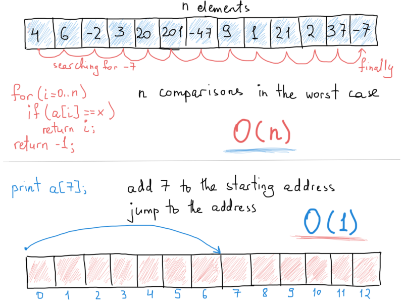
The point of “calculating” algorithmic complexity is finding a dependency between the number of operations and the size of input, for instance the array above had 100 elements and the number of operations were also 100, if the number of array elements (its input) will increase to 1423, the number of operations to find any element will also increase to 1423 (the worst case). So the thin line between input and number of operations is clear in this case, it is so-called linear, the number of operations grows as much as grows array’s input. Growth. That’s the key point in complexity, we say that searching for an element in an unsorted array takes O(N) time to emphasize that the process of finding it will take up to N operations (or even up to N operations times some constant value such as 3N). On the other hand, accessing any element in an array takes a constant time, i.e. O(1). That’s because of an array’s structure. It’s a contiguous data structure, and holds elements of the same type (mind JS arrays), so “jumping” to a particular element requires only calculating its relative position to the array’s first element.
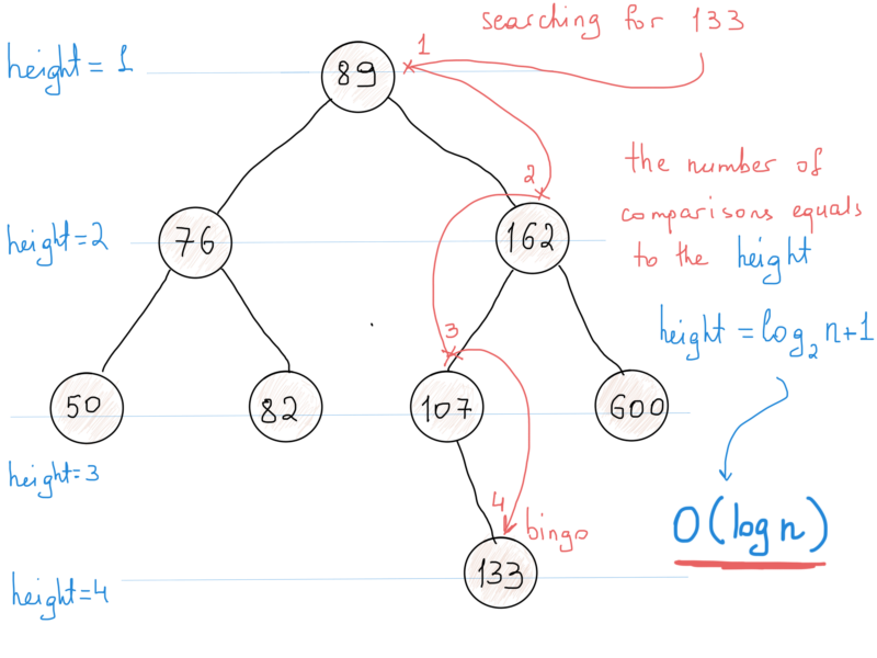
One thing is very clear. A binary search tree keeps its nodes in sorted order. So what would be the algorithmic complexity of searching an element in a binary search tree? We should calculate the number of operations required to find an element (in the worst case).
Look at the illustration above. When starting our search at the root, the first comparison may lead to three cases,
- The node is found.
- The comparison continues to node’s left sub-tree if the required element is less than the node’s value
- The comparison continues to the node’s right sub-tree if the value we search for is greater than the node’s value.
At each step we reduce the size of nodes needed to be considered by half. The number of operations (i.e. comparisons) needed to find an element in the BST equals the height of the tree. The height of a tree is the number of nodes on the longest path. In this case it’s 4. And the height is [base 2] logN + 1, as shown. So the complexity of search is O(logN + 1) = O(logN). This means that searching something in 4 million nodes requires log4000000 = ~22 comparisons in the worst case.
Back to the tree - Element access time in a binary search tree is O(logN). Why not use hashtables? Hashtables have constant access time, which makes it reasonable to use hashtables almost everywhere.
In this problem we must take into account an important requirement. We must be able to make range searches, e.g. homes with prices from $80 to $162. In case of a BST, it’s easy to get all the nodes in a range just by doing an inorder traversal of the tree and keeping a counter. For a hashtable it is somewhat expensive which makes it reasonable to stick with BSTs in this case.
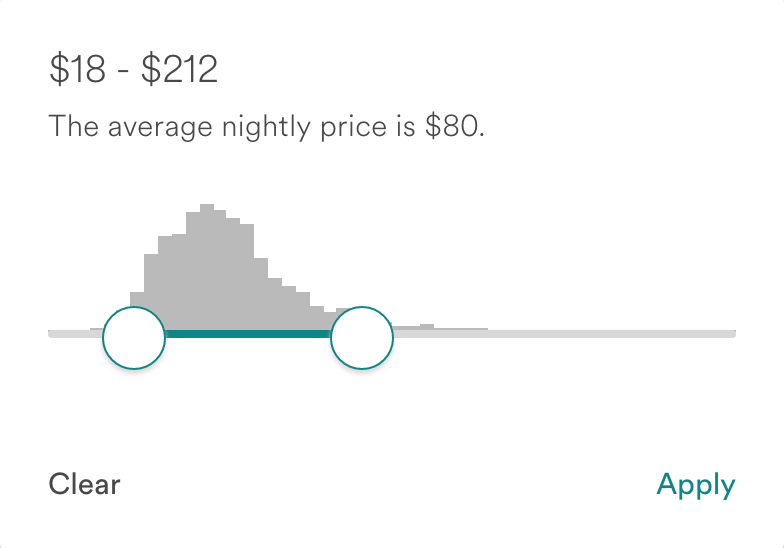
Though there is another spot, which leads us to rethink hashtables. The density. Prices won’t go up “forever”, most of the homes reside at the same price range. Look at the screenshot, the histogram shows us the real picture of the prices, millions of homes are in the same range (+/- $18 - $212), they have the same average price. Simple arrays may play a good role. Assuming the index of an array as the price and the value as the list of homes, we might access any price range in constant time (well, almost constant). Here’s how it looks (way abstract):
Just like a hashtable, we are accessing each set of homes by its price. All homes having the same price are grouped under a separate BST. It will also save us some space if we store home IDs instead of the whole object defined above (the AirbnbHome struct). The most possible scenario is to save all homes full objects in a hashtable mapping home ID to home full object and storing another hashtable (or better, an array), which maps prices with homes IDs.
So when users request a price range, we fetch home IDs from the price table, cut the results to a fixed size (i.e. the pagination, usually around 10 - 30 items are shown on one page), fetch the full home objects using each home ID.
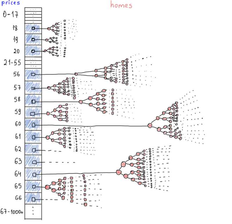
Just keep another thing in mind (think of it in the background). Balancing is crucial for a BST, because it’s the only guarantee of having tree operations done in O(logN). The problem of unbalanced BST is obvious when you insert elements in sorted order. Eventually, the tree becomes just a linked list, which obviously leads to linear-time operations. Forget this for now, suppose all our trees are perfectly balanced. Take a look at the illustration above once again. Each array element represents a big tree. What if we change the illustration to something like this:
 More like a graph
It resembles a “more realistic” graph. This illustration represents the most disguised data structures and graphs, which takes us to the next section.
Graph representation: Outro
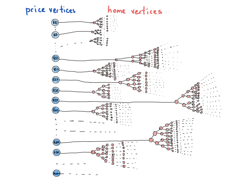
The bad news about graphs is that there isn’t a single definition for the graph representation. That’s why you can’t find a std::graph in the library. We already had a chance to represent a “special” graph called BST. The point is, tree is a graph, but graph is not a tree. The last illustration shows us that we have a lot of trees under a single abstraction, “prices vs homes” and some of the vertices “differ” in their type, prices are graph nodes having only the price value and refer to the whole tree of home IDs (home vertices) that satisfy the particular price. It is much like a hybrid data structure, than a simple graph that we’re used to seeing in textbook examples.
That’s the key point in graph representation, there isn’t a fixed and “de jure” structure for graph representation (unlike BSTs with their specified node-based representation with left/right child pointers, though you can represent a BST with a single array). You can represent a graph in the most convenient way you wish (most convenient to particular problem), the main thing is that you “see” it as a graph. And by “seeing a graph” we mean applying algorithms that are specific to graphs.
What about an N-ary tree, it is more likely to resemble a graph.
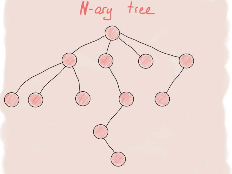
And the first thing that comes into mind to represent an N-ary tree node is something like this:
This structure represents just a single node of a tree. The full tree looks more like this:
This class is an abstraction around a single tree node named root_ . That’s all we need to build a tree of any size. That’s the starting point of the tree. For adding a new tree node we need to allocate a memory to it and add that node to the root of the tree.
A graph is much like an N-ary tree, with a slight difference. Try to spot it.
Is this a graph? No. I mean yes, but it’s the same N-ary tree from the previous illustration, just a little rotated. As a rule of a thumb, whenever you see a tree (even if it is an apple tree, lemon tree or binary search tree), you can be sure that it is also a graph. So, devising a structure for a graph node (graph vertex), we can come up with the same structure:
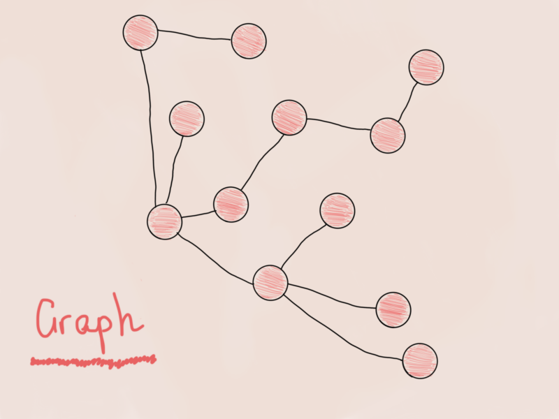
Is this enough to construct a graph? Well, no. And here’s why. Look at these two graphs from previous illustrations, find a difference:
Both are graphs
The graph in the illustration at the left side has no single point to “enter” (it’s rather a forest than a single tree), in the contrary, the graph in the right illustration doesn’t have unreachable vertices. Sounds familiar.
A graph is connected when there is a path between every pair of vertices. [Wikipedia]
Obviously, there isn’t a path between every pair of vertices for the “prices vs homes” graph (if it isn’t obvious from the illustration, just assume that prices are not connected with each other). As much as it’s just an example to show that we aren’t able to construct a graph with a single GraphNode struct, there are cases that we have to deal with disconnected graphs like this. Take a look at this class:
Just like an N-ary tree is built around a single node (the root node), a connected graph also can be built around a root node. It’s said that trees are “rooted”, i.e. they have a starting point. A connected graph can be represented as a rooted tree (with a couple of more properties), it’s already obvious, but keep in mind that the actual representation may differ from algorithm to algorithm, from problem to problem even for a connected graph. However, considering node-based nature of graphs, a disconnected graph can be represented like this:
For graph traversals like DFS/BFS it’s natural to use a tree-like representation. Helps a lot. However, cases like efficient path tracing require a different representation. Remember Euler’s graph? To track down a graph’s “eulerness”, we should trace an Euler path within it. That means visiting all vertices by traversing each edge only once, and when the tracing finishes and we have untraversed edges, then the graph doesn’t have an Euler path, and therefore is not an Euler graph.
There is even faster method, we can check the degrees of vertices (suppose each vertex stores its degree) and just as the definition says, if a graph has vertices of odd degree and there aren’t exactly two of them, then it is not an Euler graph. The complexity of such a check is O(|V|), where |V| is the number of graph vertices. We can track down odd/even degrees while inserting new edges to increase odd/even degree checks to O(1). Lightning fast. Never mind, we’re just going to trace a graph, that’s it. Below is both the representation of a graph and the Trace() function returning a path.
Mind the bugs, bugs are everywhere. This code contains a lot of assumptions, for instance, the labeling, so by a vertex we understand a string label. Sure you can easily update it to be anything you want. Doesn’t matter in the context of this example. Next, the naming. As mentioned in the comments, VELOGraph is for Vertex Edge Label Only Graph (I made this up). The point is, this graph representation contains a table for mapping a vertex label with edges incident to that vertex, and a list of edges containing a pair of vertices (connected by a particular edge) and a flag which is used only by the Trace() function. Take a look at the Trace() function implementation. It uses edge’s flag to mark an already traversed edge (flags should be reset after any Trace() call).
Twitter Example: Tweet Delivery Problem
Here’s another representation called an adjacency matrix, which could be useful in directed graphs, like one we used for Twitter follower graph.
Directed graph
There are 8 vertices in this Twitter example. So all we need to represent this graph is a |V|x|V| square matrix (|V| number of rows and |V| number of columns). If there is a directed edge from v to u, then matrix’s [v][u] is true, otherwise it’s false.
 Twitter’s example
As you can see, this matrix is way too sparse, its trade off is the fast access. To see if Patrick follows Sponge Bob, we should just check the value of matrix["Patrick"]["Sponge Bob"]. To get the list of Ann’s followers, we just process the entire “Ann” column (title is in yellow). To find who are being followed (sounds strange) by Sponge Bob, we process the entire row “Sponge Bob”. Adjacency matrix could be used for undirected graphs as well, and instead of settings 1’s if a there is an edge from v to u, we should set both values to 1, e.g. adj_matrix[v][u] = 1, adj_matrix[u][v] = 1. Undirected graph’s adjacency matrix is symmetric.
Note that instead of storing ones and zeroes in an adjacency matrix, we can store something “more useful”, like edge weights. One of the best examples might be a graph of places with distance information.
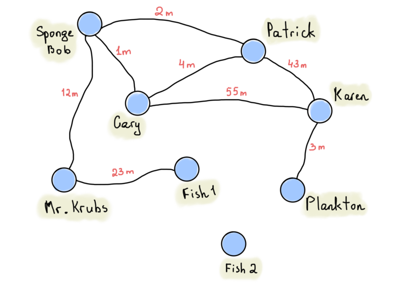
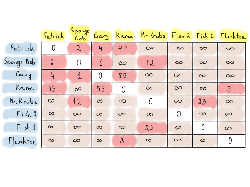
The graph above represents distances between houses of Patrick, Sponge Bob and others (also known as weighted graph). We put “infinity” signs if there isn’t a direct route between vertices. That doesn’t mean that there are no routes at all, and at the same time that doesn’t mean that there must necessarily be routes. It might be defined while applying an algorithm for finding a route between vertices (there is even better way to store vertices and edges incident to it, called an incidence matrix).
 _82000Tb. [Photo source](http://www.independent.co.uk/arts-entertainment/tv/news/the-simpsons-death-episode-will-be-bigger-than-game-of-thrones-9304810.html" rel="noopener" target="blank" title=")
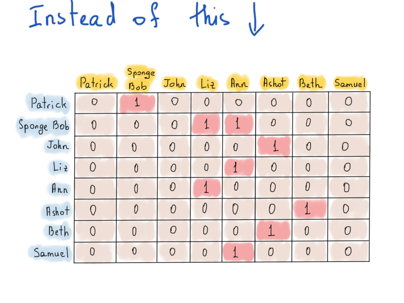
While adjacency matrix seemed a good use for Twitter’s followes graph, keeping a square matrix for nearly 300 million users (monthly active users) takes 300 300 1 bytes (storing boolean values). That is, ~82000 Tb (Terabytes), which is 1024 * 82000 Gb. Well, don’t know about your home cluster, my laptop doesn’t have so much RAM. Bitsets? A BitBoard could help us a little, reducing the required size to ~10000 Tb. Still way too big. As mentioned above, an adjacency matrix is too sparse. It forces us to use more space than actually needed. That’s why using a list of edges incident to vertices may be useful. The point is, an adjacency matrix allows us to keep both “follows” and “doesn’t follow” information, while all we need is to know information about the followes, something like this:
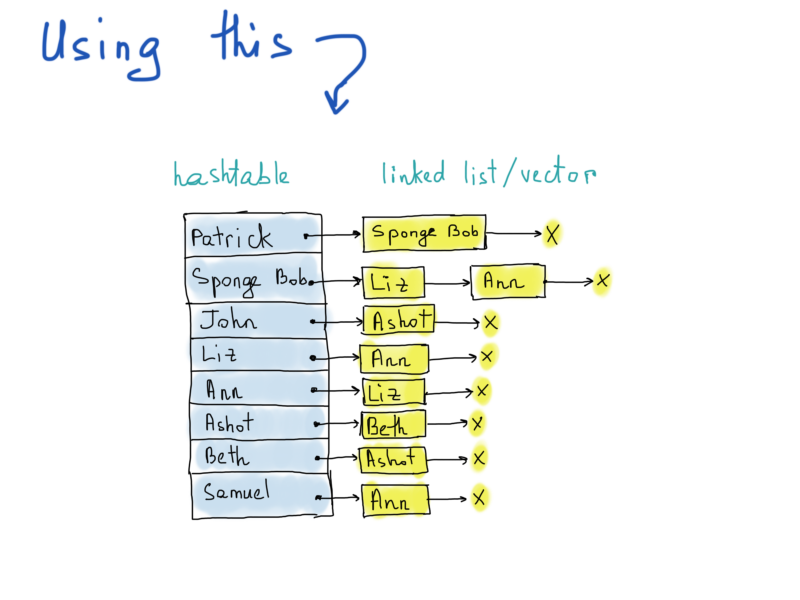 Adjacency matrix vs adjacency list
The illustration at the right side is called an adjacency list. Each list describes the set of neighbors of a vertex in the graph. By the way, the actual implementation of the graph representation as an adjacency list, again, differs (ridiculous facts). In the illustration, we highlighted a hashtable usage, which is reasonable, as the access of any vertex will be O(1), and for the list of neighbor vertices we didn’t mention the exact data structure, deviating from linked lists to vectors. Choice is yours.
The point is, to find out whether Patrick does follow Liz, we should access the hashtable (constant time) and go through all items in the list comparing each element with “Liz” element (linear time). Linear time isn’t that bad at this point, because we have to loop over only a fixed amount of vertices adjacent to “Patrick”. What about the space complexity, is it ok to use at Twitter? Well, we need at least 300 million hashtable records, each of which points to a vector (choosing vector to avoid memory overhead of linked lists’ left/right pointers) containing, how much? No stats here, found just an average number of twitter followers, 707 (googled).
So if we consider that each hashtable record points to an array of 707 user IDs (each weighing 8 byte), and let’s assume that hashtable’s overhead is only its keys, which are again, user ids, so the hashtable itself takes 300 million 8 bytes. Overall, we have 300 million 8 bytes for hashtable + 707 8 bytes for each hashtable key, that is 300 million 8 707 8 bytes = ~12 Tb. Well, can’t say that feels better, but yes, feels much better than 10,000 Tb.
Honestly, I don’t know whether this 12Tb is a reasonable number. But considering the fact that I’m spending around $30 on a dedicated server machine with 32 Gb of RAM, then, storing (sharded) 12 Tb requires at least 385 such servers, plus a couple of control servers (for data distribution control) rounds up to 400. So it will cost me $12K (monthly).
Well, considering the fact that the data should be replicated, and that something always can go wrong, we’ll triple the number of servers and then again, add some control servers, let’s say we need at least 1500 servers, which will cost us $45K monthly. Well, definitely not good for me as I hardly can keep one server, but seems okay for Twitter (it’s really nothing compared to real Twitter servers). Let’s assume it is really okay for Twitter.
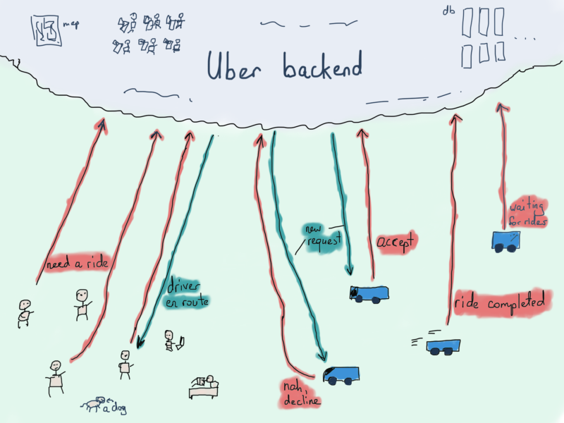
Now, are we okay here? Not yet, that was just the data regarding the followers. What is the main thing in Twitter? I mean, technically, what is its biggest problem? You won’t be alone if you say it’s the fast delivery of tweets. I will definitely second that. And not fast, but lightning fast. Say Patrick tweeted something about his thoughts on food, all his followers should receive that very tweet in a reasonable time. How long will it take? We are free of making any assumption here, and use any abstractions we want, but we are interested in the real world production systems, so, let’s dig. Here’s what’s typically happens when someone tweets.
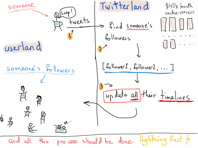
Again, don’t know much about how long it takes for one tweet to reach all followers, but publicly available statistics tell us that there are about 500 million daily tweets. Daily! ?
So the process above happens 500 million times every day. I can’t really find anything on tweet delivery speed. I vaguely recall something about a maximum of 5 seconds for a tweet to reach all its followers. And also note the “heavy cases”, celebrities with more than a million followers. They might tweet something about their wonderful breakfast at the beach house, but Twitter sweats much to deliver that super-useful content to millions of followers.
To solve tweet delivery problem we don’t really need the graph of followers, instead we need a graph of followers. The previous graph (with a hashtable and a bunch of lists) allows us to efficiently find all users followed by any particular user. But it does not allow us to efficiently find all users who are following one particular user, for that case we have to scan all the hashtable keys. That’s why we should construct another graph, which is kind of a symmetric opposite to the one we constructed for followers. This new graph will again consist of a hashtable containing all 300 million vertices, each of which points to a list of adjacent vertices (the structure remains the same), but this time, the list of adjacent vertices will represent followers.
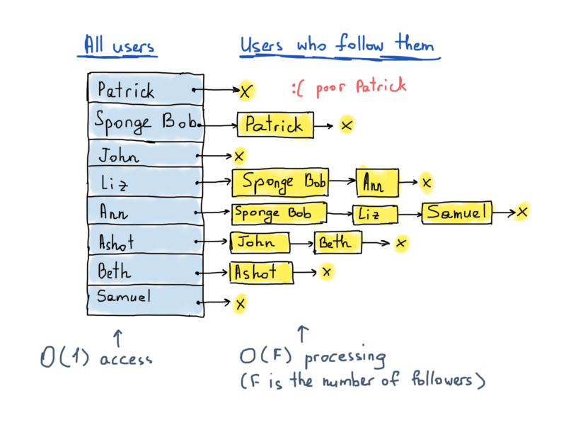
So based on this illustration, whenever Liz tweets something, Sponge Bob and Ann must see that very tweet on their timelines. A common technique to accomplish this is by keeping separate structures for each user’s timeline. In case of Twitter’s 300+ million users, we might assume there are at least 300+ million timelines (for each user). Basically, whenever a user tweets, we should get the list of user’s followers and update their timelines (insert that same tweet into each one of them). A timeline might be represented as a linked list, or a balanced tree (tweet datetimes as node keys).
This is just a basic idea we abstracted from actual timeline representation and of course, we can make the actual delivery faster if we use multithreading. This is crucial for ‘heavy cases’, because for millions of followers the ones that reside closer to the end are being processed later than the ones residing closer to the front of the list.
The following pseudocode tries to illuminate this multithreading delivery idea:
So whenever followers refresh their timelines, they will receive the new tweet.
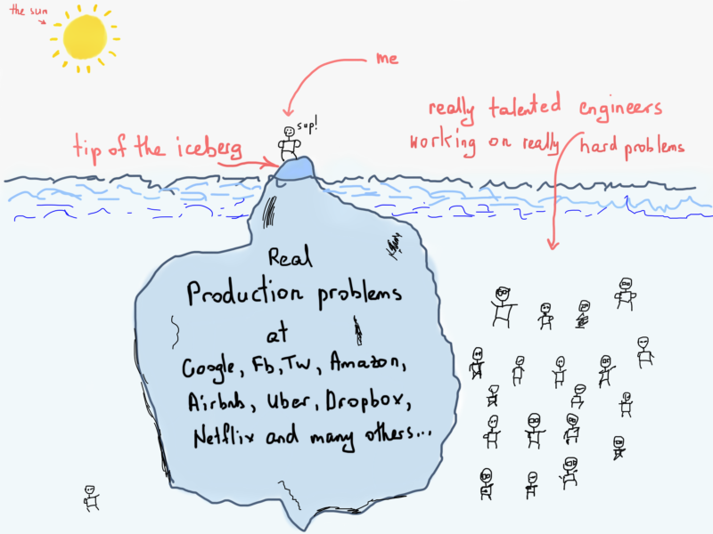
It will be fair to say, that we merely touched the tip of the iceberg of real problems at Airbnb or Twitter. It takes a really long time and the hard work of really talented engineers to accomplish such great results in complex systems like Twitter, Google, Facebook, Amazon, Airbnb and others. Just keep this in mind while reading this article.
The point of demonstrating Twitter’s tweet delivery problem is to embrace the usage of graphs, even though we didn’t use any graph algorithm, we just used a representation of the graph. Sure we pseudocoded a function for delivering tweets, but that is something we came up during the process of searching for a solution.
What I meant by “any graph algorithm” is any algorithm from this list. As something big enough to make programmers cry, graph theory and graph algorithm applications are somewhat different to spot at a glimpse. We were discussing the Airbnb homes and efficient filtering before finishing with graph representations, and the main obvious thing was the inability to efficiently filter homes with more than one filter key. Is there anything that could be done using graph algorithms? Well, we can’t tell for sure, but at least we can try. What if we represent each filter as a separate vertex?
Literally each filter, even all the prices from $10 to $1000+, all city names, country codes, amenities (TV, Wi-Fi, and all others), number of adults, and each number as a separate graph vertex.
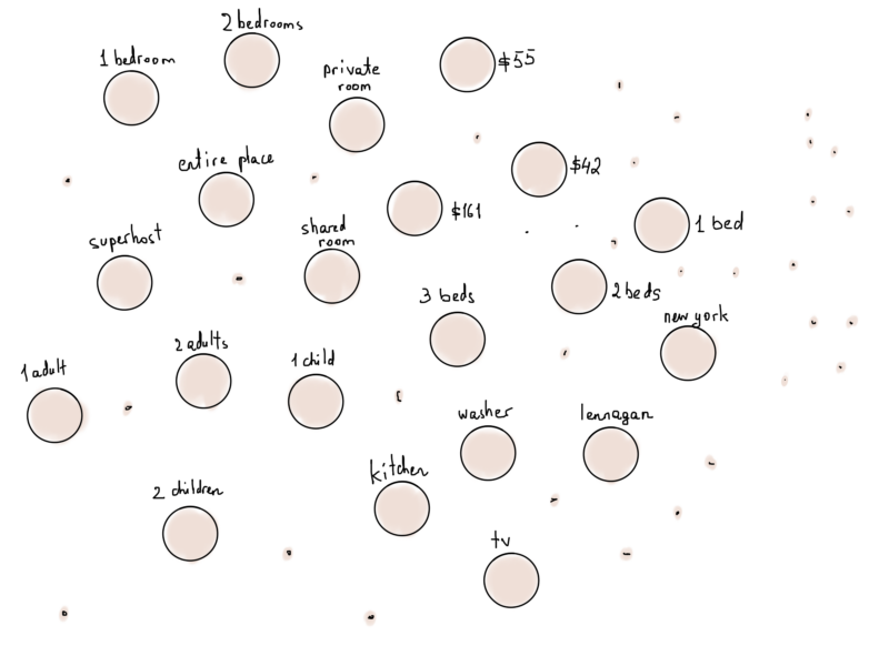 Excerpt of Airbnb filters
We can even make this set of vertices more “friendly” if we add “type” vertices too, like “Amenities” connected to all vertices representing an amenity filter.
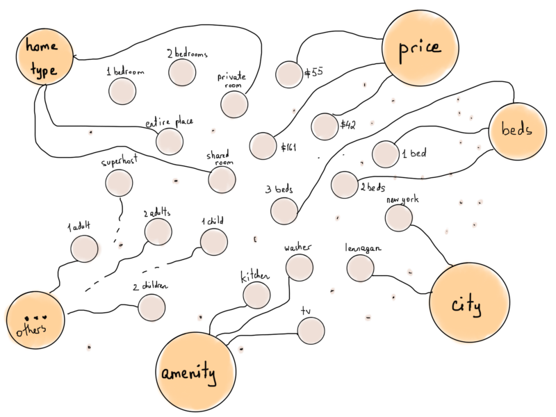 Airbnb filters with types
Now, what if we represent Airbnb homes as vertices and then connect each home with “filter” vertex if that home supports the corresponding filter (For example, connecting “home 1” with “kitchen” if “home 1” has “kitchen” in its amenities)?
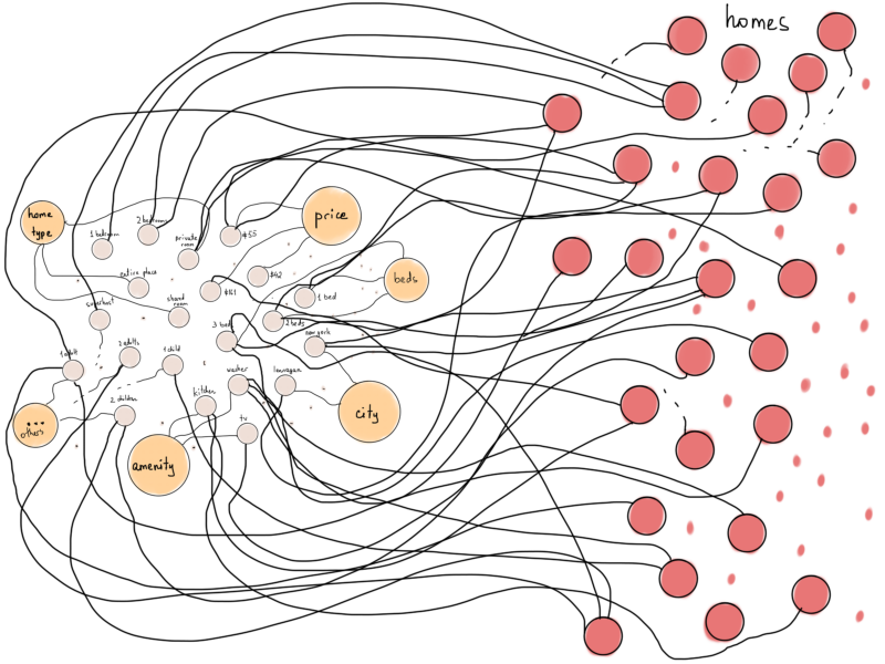 Looks messy
A subtle change of this illustration makes it more likely to resemble a special type of graph, called a bipartite graph.
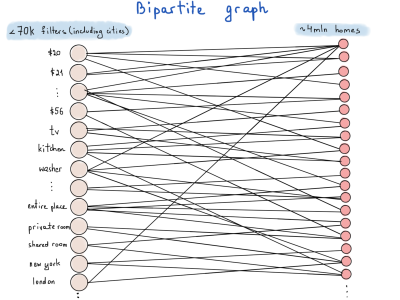 Number of vertices are more than it may appear
_Bipartite graph or just bigraph is a graph whose vertices can be divided into two disjoint and independent sets such that every edge connects a vertex in one set to one in other set. - Wikipedia_.
In our example one of the sets represents filters (we’ll denote it by F) and the other is a homes set (denoted by H). For example, if there are 100 thousand homes with the price value $62, then price vertex labeled “$62” will have 100 thousand edges incident to each homes vertices. If we measure the worst case of space complexity, i.e. each home has all the properties satisfying to all the filters, than the total amount of edges to be stored will be 70,000 4 million. If we represent each edge as a pair of two ids: {filter_id; home_id} and if we rethink about IDs and use a 4 byte (int) numeric id for filters and 8 byte (long) id for homes, then each edge would require at least 12 bytes. So storing 70,000 4 million 12 bytes values will require around 3Tb of memory. We made a small mistake in calculation, you see.
The number of filters is around 70,000 because of the 65 thousand cities active in Airbnb (stats). And the good news is that the same home cannot be located in more than one city. That is, our actual number of edges pairing with cities is 4 million (each home located in one city). So we’ll calculate for 70k - 65k = 5 thousand filters, that means we need 5000 4 million 12 bytes of memory, which is less than 0.3 Tb. Sounds good. But what gives us this bipartite graph? Most commonly a website/mobile request will consist of several filters, for example like this:
house_type: "entire_place",adults_number: 2,price_range_start: 56,price_range_end: 80,beds_number: 2,amenities: ["tv", "wifi", "laptop friendly workspace"],facilities: ["gym"]
And all we need is to find all the “filter vertices” above and process all the “home vertices” that are adjacent to these “filter vertices”. This takes us to a scary subject.
Graph Algorithms: Intro
Any processing done with graphs might be categorized as a “graph algorithm”. You literally can implement a function printing all the vertices of a graph and name it “_’s vertex printing alg_orithm”. Most of us are scared of the graph algorithms listed in textbooks (see the full list here). Let’s try to apply a bipartite graph matching algorithm, such as Hopcroft-Karp algorithm to our Airbnb homes filtering problem:
Given a bipartite graph of Airbnb homes (H) and filters (F), where every element (vertex) of H can have more than one adjacent elements (vertex) of F (sharing a common edge). Find a subset of H consisting of vertices that are adjacent to vertices in a subset of F.
Confusing problem definition, however we can’t be sure at this point whether Hopcroft-Karp algorithm solves our problem. But I assure you that this journey will teach us many crucial ideas behind graph algorithms. And the journey is not so short, so be patient.
_The Hopcroft–Karp algorithm is an algorithm that takes as input, a bipartite graph and produces as output, a maximum cardinality matching - a set of as many edges as possible with the property that no two edges share an endpoint - Wikipedia._
Readers familiar with this algorithm are already aware that this doesn’t solve our problem, because matching requires that no two edges share a common vertex.
Let’s look at an example illustration, where there are just 4 filters and 8 homes (for the sake of simplicity).
- Homes are denoted by letters from A through H, filters are chosen randomly.
- Home A has a price ($50), and 1 bed, (that’s all we got for the price).
- All homes from A through H have a $50 per night price tag and 1 bed, but few of them have “Wi-Fi” and/or “TV”.
So the following illustration tries to show which homes should we “return” for the request asking for homes that have all four filters available (For example, they cost $50 per night, they have 1 bed and also they have Wi-Fi and TV).
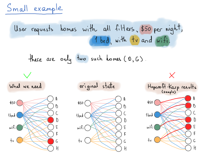
The solution to our problem requires edges with common vertices leading to distinct home vertices that are incident to the same filter subset, while Hopcroft-Karp algorithm eliminates such edges with common endpoints and produces edges incident to vertices in both subsets.
Take a look at the illustration above, all we need are homes D and G, which both satisfy to all four filter values. What we really need is to get all matching edges which share a common endpoint.
We could devise an algorithm for this approach, but its processing time is arguably not relevant to users needs (users needs = lightning fast, right here, right now). Probably it would be faster to create a balanced binary search tree with multiple sort keys, almost like a database index file, which maps primary/foreign keys with a set of satisfying records.
Balanced binary search trees and database indexing will be discussed in a separate article, where we will return to the Airbnb home filtering problem again.
The Hopcroft-Karp algorithm (and many others) are based on both DFS (Depth-First Search) and BFS (Breadth-First Search) graph traversal algorithms. To be honest, the actual reason to introduce the Hopcroft-Karp algorithm here is to surreptitiously switch to graph traversals, which is better to start from the nice graphs, binary trees.
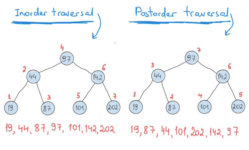
Binary tree traversals are really beautiful, mostly because of their recursive nature. There are three basic traversals called in-order, post-order and pre-order (you may come up with your own traversal algorithm). They are easy to understand if you have ever traversed a linked list. In linked lists you just print the current node’s value (named item in the code below) and continue to the next node.
Almost the same goes with binary trees, you print the node value (or whatever else you need to do with it) and then continue to the next node, but in this case, there are “two next” nodes, left and right. So you should do the same for both left and right nodes. But you have three different choices here:
- print the node value then go to the left node, and then go to the right node, or
- go to the left node, print the node value, and then go to the right node, or
- go to the left node, then go to the right node, and then print the value of the node.
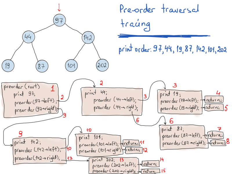 Detailed tracing of pre-order traversal
Obviously, recursive functions look very elegant though they are so expensive. Each time we call a function recursively, it means we call a completely “new” function (see the illustration above). And by “new” we mean that another stack memory space should be “allocated” for the function arguments and local variables. That’s why recursive calls are expensive (the extra stack space allocations and the many function calls) and dangerous (mind the stack overflow) and it is obviously suggested to use iterative implementations. In mission critical systems programming (aircraft, NASA rovers and so on) a recursion is completely prohibited (no stats, no experience, just telling you the rumors).
Netflix and Amazon: Inverted Index Example
Let’s say we want to store all Netflix movies in a binary search tree with movie titles as sort keys. So whenever a user types something like “Inter”, we will return a list of movies starting with “Inter” (for instance, “Interstellar”, “Interceptor”, “Interrogation of Walter White”).
Now, it would be great if we’ll return every movie that contains “Inter” in its title (not only ones that start with “Inter”), and the list would be sorted by movie ratings or something that is relevant to that particular user (like thrillers more than drama). The point of this example is to make efficient range queries to a BST.
But as usual, we won’t dive deeper into the cold water to spot the rest of the iceberg. Basically, we need a fast lookup by search keywords and then get a list of results sorted by some key, which most likely should be a movie rating and/or some internal ranking based on a user’s personalized data. We’ll try to stick to the KISK principle (Keep It Simple, Karl) as much as possible.
“KISK” or “let’s keep it simple” or “for the sake of simplicity”, a super excuse for tutorial writers to abstract from the real problem and make tons of assumptions by bringing an “abc” easy example and its solution in pseudocode that works even on your grandma’s laptop.
This problem could be easily applied to Amazon’s product search as we most commonly search something in Amazon by typing a text describing our interest (like “Graph Algorithms”) and get results sorted by product ratings. I haven’t experienced personalized results in Amazon’s search results. But I’m pretty sure Amazon does that stuff too. So, it will be fair to change the title of this subtopic to…
Netflix and Amazon. Netflix serves movies, Amazon serves products, we’ll name them “items”, so whenever you read an “item” think of a movie in Netflix or any [viable] product in Amazon.
What is most commonly done with the items is the parsing of their title and description (we’ll stick to the title only), so if an operator (usually a human being inserting item’s data into Netflix/Amazon database via an admin dashboard) inserts a new item into the database, its title is being processed by some “ItemTitleProcessor” to produce keywords.
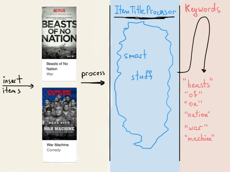 Not the best illustration, I know (and has a typo)
Each item has its unique ID, which is being linked to the keyword found in its title. This is what search engines do while crawling websites all over the world. They analyze each document’s content, tokenize it (break it into smaller entities called words) and add it to a table, which maps each token (word) to the document ID (website) where the token has been “seen”.
So whenever you search for “hello”, the search engine fetches all documents mapped to the keyword “hello” (reality is much complex, because the most important thing is the search relevancy, which is why Google Search is so awesome). So a similar table for Netflix/Amazon may look like this (again, think of Movies or Products when reading Items).
 Inverted index
Hashtables, again. Yes, we will keep a hashtable for this inverted index (_index structure storing a mapping from content - Wikipedia_). The hashtable will map a keyword to a BST of items. Why BST? Because we want to keep them sorted and at the same time serve them (respond to frontend requests) in sequential sorted portions, (for instance, 100 items at a request using pagination). Not really something that shows the power of BSTs. But let’s pretend that we also need a fast lookup in the search result, say you want all 3 star movies with the keyword “machine”.
Note that it’s okay to have duplicate items in different trees, because an item usually can be found with more than one keyword.
We’ll operate with items defined as follows:
Each time a new item is inserted into a database, the title is processed and added to the big index table, which maps a keyword to an item. There could be many items sharing the same keyword, so we keep these items in a BST sorted by their rating.
When users search for some keyword, they get a list of items sorted by their rating. How can we get a list from a tree in a sorted order? By doing an in-order traversal.
Here’s how an implementation of InOrderProduceVector() might look:
But, but… We need the highest rated items first, and our in-order traversal produces the lowest rated items first. That’s because of its nature. In-order traversal works “bottom up”, from the lowest to the highest item. To get what we wanted, i.e. the list in descending order instead of ascending, we should take a look at the in-order traversal implementation a bit closer.
What we are doing is going through the left node, then printing the current node’s value and then going through the right node. The left most node is the node with the smallest value. So simply changing the implementation to go through the right node first will lead us to a descending order of the list. We’ll name it as others do, a reverse in-order traversal.
Let’s update the code above (introducing in a single listing). Warning - Bugs Ahead!
That’s it. We can serve item search results pretty fast. As mentioned above, inverted indexing is used mostly in search engines, like Google. Although Google Search is a very complex search engine, it does use some simple ideas (way too modernized though) to match search queries to documents and serve the results as fast as possible.
We used tree traversals to serve results in sorted order. At this point it might seem that pre/in/post-order traversals are more than enough, but sometimes there is a need for another type of traversal.
Let’s tackle this well-known programming interview question, “How would you print a [binary] tree level by level?”.
Traversals: DFS and BFS
If you are not familiar with this problem, think of some data structure that you could use to store nodes while traversing the tree. If we compare level-by-level traversal of a tree with the others above (pre, in, post order traversals), we’ll eventually devise two main traversals of graphs, that is a depth-first search (DFS) and breadth-first search (BFS).
Depth-first search hunts for the farthest node, breadth-first search explores nearest nodes first.
- Depth-first search - more actions, less thoughts.
- Breadth-first search - take a good look around you before going farther.
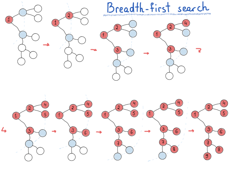
DFS is much like pre, in, post-order traversals. While BFS is what we need if we want to print a tree’s nodes level-by-level.
To accomplish this, we would need a queue (data structure) to store the “level” of the graph while printing (visiting) its “parent level”. In the previous illustration nodes that are placed in the queue are in light blue.
Basically, going level by level, nodes on each level are fetched from the queue, and while visiting each fetched node, we also should insert its children into the queue (for the next level). The following code is simple enough to get the main idea of BFS. It is assumed that the graph is connected, although it can be modified to apply to disconnected graphs.
The basic idea is easy to show on a node-based connected graph representation. Just keep in mind that the implementation of the graph traversal differs from representation to representation.
BFS and DFS are important tools in tackling graph searching problems (but remember that there are tons of graph search algorithms). While DFS has elegant recursive implementation, it is reasonable to implement it iteratively. For the iterative implementation of BFS we used a queue, for DFS you will need a stack. One of the most popular problems in graphs and at the same time one of the most possible reasons you read in this article is the problem of finding the shortest path between graph vertices. And this takes us to our last thought experiment.
Uber and the Shortest Path Problem (Dijkstra’s Algorithm)
With its 50 million users and 7 million drivers (source), one of the most important things that is critical to Uber’s functioning is the ability to match drivers with riders in an efficient way. The problem starts with locations.
The backend should process millions of user requests, sending each of the requests to one or more (usually more) drivers nearby. While it is easier and sometimes even smarter to send the user request to all nearby drivers, some pre-processing might actually help.
Besides processing incoming requests and finding the location area based on the user coordinates and then finding drivers with nearest coordinates, we also need to find the right driver for the ride. To avoid geospatial request processing (fetching nearby cars by comparing their current coordinates with user’s coordinates), let’s say we already have a segment of the map with user and several nearby cars.
Something like this:
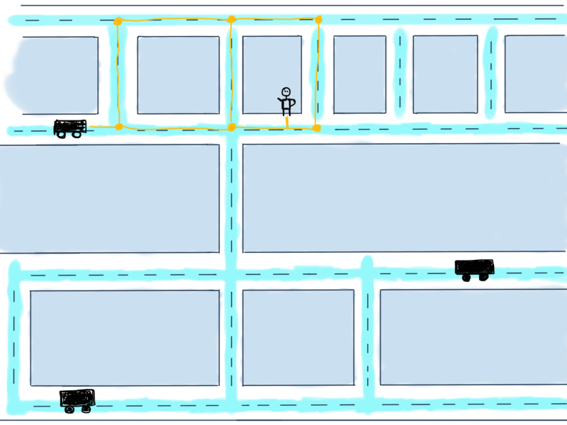
Possible paths from a car to a user are in yellow. The problem is to calculate the minimum required distance for the car to reach the user, in other words, find the shortest path between them. While this is more about Google Maps rather than Uber, we’ll try to solve it for this particular and very simplified case mostly because there are usually more than one drivers car and Uber might want to calculate the nearest car with the highest rating to send it to the user.
For this illustration that means calculating for all three cars the shortest path reaching to the user and decide which car would be the optimal to send. To make things really simple, we’ll discuss the case with just one car. Here are some possible routes to reach to the user.
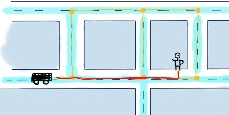
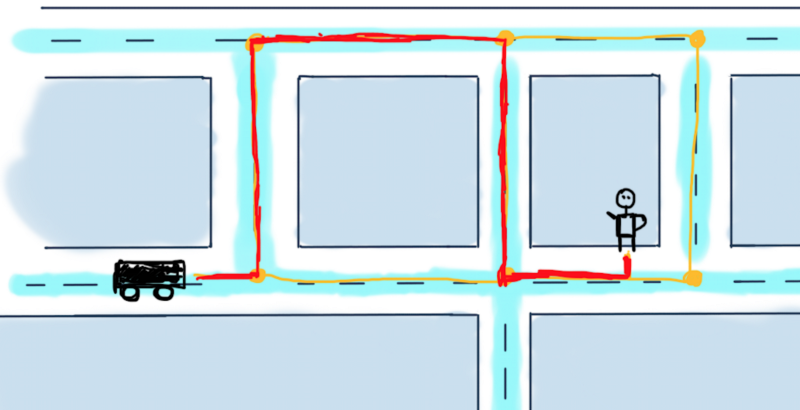
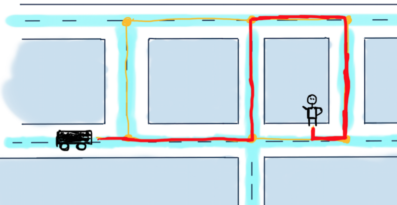 Possible variants to reach the user
Cutting to the chase, we’ll represent this segment as a graph:
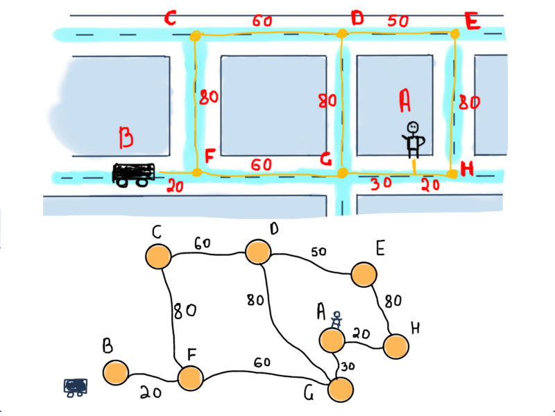
This is an undirected weighted graph (edge-weighted, to be more specific). To find the shortest path between vertices B (the car) and A (the user), we should find a route between them consisting of edges with possibly minimum weights. You are free to devise your version of the solution. We’ll stick with Dijkstra’s version. The following steps of Dijkstra’s algorithm are from Wikipedia.
Let the node at which we are starting be called the initial node. Let the distance of node Y be the distance from the initial node to Y. Dijkstra’s algorithm will assign some initial distance values and will try to improve them step by step.
- Mark all nodes unvisited. Create a set of all the unvisited nodes called the unvisited set.
- Assign to every node a tentative distance value: set it to zero for our initial node and to infinity for all other nodes. Set the initial node as current.
- For the current node, consider all of its unvisited neighbors and calculate their tentative distances through the current node. Compare the newly calculated tentative distance to the current assigned value and assign the smaller one. For example, if the current node A is marked with a distance of 6, and the edge connecting it with a neighbor B has length 2, then the distance to B through A will be 6 + 2 = 8. If B was previously marked with a distance greater than 8 then change it to 8. Otherwise, keep the current value.
- When we are done considering all of the neighbors of the current node, mark the current node as visited and remove it from the unvisited set. A visited node will never be checked again.
- If the destination node has been marked visited (when planning a route between two specific nodes) or if the smallest tentative distance among the nodes in the unvisited set is infinity (when planning a complete traversal; occurs when there is no connection between the initial node and remaining unvisited nodes), then stop. The algorithm has finished.
- Otherwise, select the unvisited node that is marked with the smallest tentative distance, set it as the new “current node”, and go back to step 3.
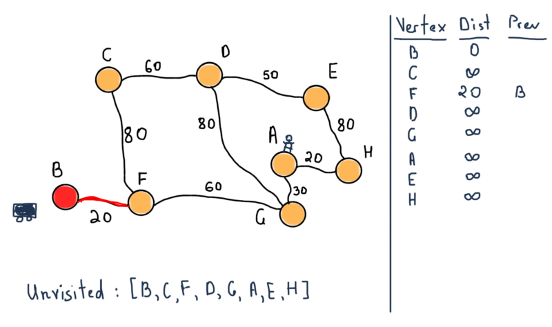
Applying this to our example, we’ll start with vertex B (the car) as the initial node. For first two steps:
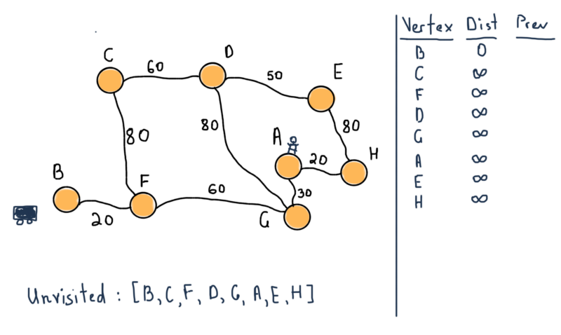
Our unvisited set consists of all vertices. Also note the table at the left side of the illustration. For all vertices, it will contain all the shortest distances from B and the previous (marked “Prev”) vertex that lead to the vertex. For instance the distance is 20 from B to F, and the previous vertex is B.
We are marking B as visited and move it to its neighbor F.
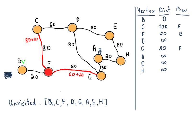
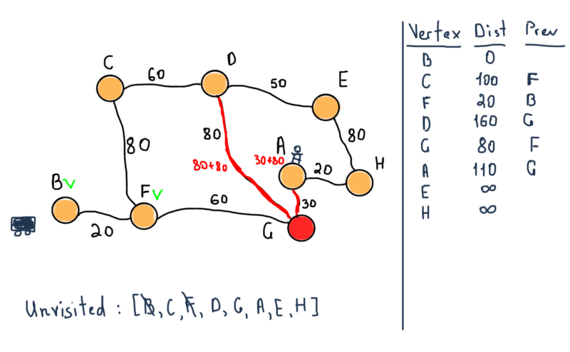
Now we are marking F as visited and choosing the next unvisited node with smallest tentative distance, which is G. Also note the table at the left side. In the previous illustration nodes C, F and G already have their tentative distances set with the previous nodes which lead to the mentioned nodes.
As stated in the algorithm, if the destination node has been marked visited (when planning a route between two specific nodes as in our case) then we can stop. So our next step stops the algorithm with the following values.
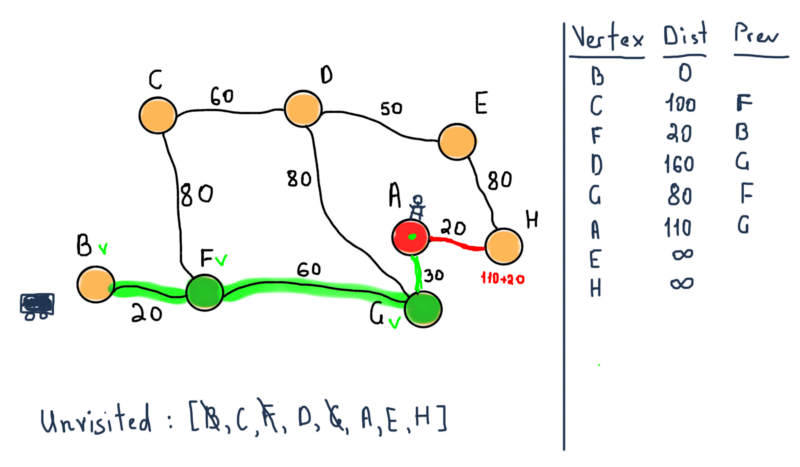
So we have both the shortest distance from B to A and the route through F and G nodes.
This is really the simplest possible example of potential problems at Uber, comparing this to our iceberg analogy, we are at the tip of the tip of the iceberg. However, this is a good first start to explore the real world of graph theory and its applications. I didn’t complete what I initially planned for in this article, but in the near future, most probably, this will be continued (also including database indexing internals).
There is still so much to tell about graphs (still need to study). Take this article as another tip of the iceberg. If you have read this far, you definitely deserve a cookie. Don’t forget to clap and share. Thank you.
Resources
[1] Sh. Even, G. Even, Graph Algorithms
Further reading
R. Sedgewick, K. Wayne, Algorithms
T. Cormen, Ch. Leiserson, R. Rivest, C. Stein, Introduction to Algorithms
Airbnb Engineering, AirbnbEng
Netflix Tech Blog, Netflix Technology Blog