
By Davis David
When you're training a machine learning model, you can have some features in your dataset that represent categorical values. Categorical features are types of data that you can divide into groups.
There are three common categorical data types:
- Ordinal – a set of values in ascending or descending order. Example: rating happiness on a scale of 1-10
- Binary – a set with only two values. Example: hot or cold.
- Nominal – a set containing values without a particular order. Example: a list of countries
Most machine learning algorithms require numerical input and output variables. This means that you will have to transform categorical features in your dataset into integers or floats so the machine learning algorithms can use them.
You can either use LabelEncoding for the binary features or the One-hot-encoding method for nominal features.
In this article, you will learn how combining categorical features can improve your machine learning model's performance.
So let’s get started. 🚀
How to Combine Categorical Features in Machine Learning Models
You can create a new feature that is a combination of the other two categorical features. You can also combine more than three or four or even more categorical features.
df["new_feature"] = (
    df.feature_1.astype(str)
     + "_"
     + df.feature_2.astype(str)
    )
In the above code, you can see how you can combine two categorical features by using Pandas and form a new feature in your dataset.
So which categorical features should you combine? Well, there isn't an easy answer to that. It depends on your data and the types of features. Some domain knowledge might be useful for creating new features like this.
To illustrate the whole process, we are going to use the Financial Inclusion in Africa dataset from the Zindi competition page. It has many categorical features that we can combine to see if we can improve the model's performance.
The objective of this dataset is to predict who is most likely to have a bank account. So this is a classification problem.
Step 1 – Load the Dataset
Our first step is to make sure that we have downloaded the dataset provided in the competition. You can download the dataset here.
Import the important Python packages like this:
import pandas as pd
import numpy as np
import matplotlib.pyplot as plt
import seaborn as sns
import warnings
np.random.seed(123)
warnings.filterwarnings('ignore')
%matplotlib inline
Then load the dataset.
# Import data
data = pd.read_csv('data/Train_v2.csv')
Let’s look at the shape of our dataset:
# print shape
print('data shape :', data.shape)

data shape : (23524, 13)
The above output shows the number of rows and columns in the dataset. We have 13 variables in the dataset – 12 independent variables, and 1 dependent variable.
We can see the first five rows from our data set by using the head() method from the Pandas library.
# inspect data

data.head()
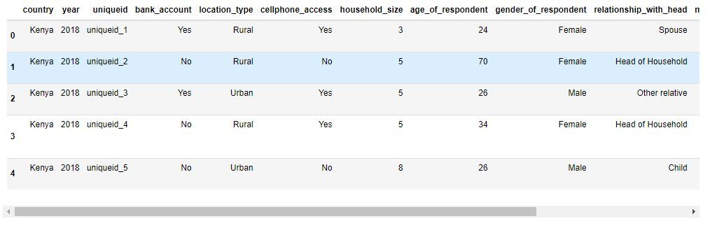
It is important to understand the meaning of each feature so you can really comprehend the dataset. You can read the VariableDefinition.csv file to understand the meaning of each variable presented in the dataset.
Step 2 – Interpret the Dataset
We can get more information about the features we have by using the info() method from Pandas.
#show Some information about the dataset

print(train_data.info())
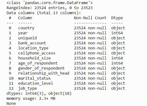
The output shows the list of variables/features, sizes if it contains missing values, and data type for each variable.
We don’t have any values missing from the dataset. We have three features of integer data type and 10 features of the object data type (most are categorical features).
Step 3 – Prepare the Data for the Machine Learning Models
The next step is to separate the independent variables and target (bank_account) from the data. Then transform the target values from the object data type into numerical using LabelEncoder.
#import preprocessing module
from sklearn.preprocessing import LabelEncoder
from sklearn.preprocessing import MinMaxScaler

# Convert target label to numerical Data
le = LabelEncoder()
data['bank_account'] = le.fit_transform(data['bank_account'])

#Separate training features from target
X = data.drop(['bank_account'], axis=1)
y = data['bank_account']

print(y)
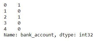
We've transformed the target values into numerical data types – 1 represents ‘Yes’ and 0 represents ‘No’.
I have created a simple preprocessing function to:
- Handle conversion of data types.
- Convert categorical features to numerical features by using One-hot Encoder and/or Label Encoder.
- Drop the uniqueid variable.
- Perform feature scaling.
# function to preprocess our data

def preprocessing_data(data):

    # Convert the following numerical labels from interger to float
    float_array = data[["household_size", "age_of_respondent", "year"]].values.astype(float
    )

    # categorical features to be converted to One Hot Encoding
    categ = [
        "relationship_with_head",
        "marital_status",
        "education_level",
        "job_type",
        "country",
    ]

    # One Hot Encoding conversion
    data = pd.get_dummies(data, prefix_sep="_", columns=categ)

    # Label Encoder conversion
    data["location_type"] = le.fit_transform(data["location_type"])
    data["cellphone_access"] = le.fit_transform(data["cellphone_access"])
    data["gender_of_respondent"] = le.fit_transform(data["gender_of_respondent"])

    # drop uniquid column
    data = data.drop(["uniquid"]), axis=1)

    # scale our data
    scaler = StandardScaler()
    data = scaler.fit_transform(data)

    return data
Let’s preprocess our dataset.
# preprocess the train data
processed_test_data = preprocessing_data(X_train)
Step 4 – Model Building and Experiments
We'll use a portion of the data set to evaluate our models.
# Split train_data
from sklearn.model_selection import train_test_spilt
X_Train, X_val, y_Train, y_val = train_test_split(processed_train_data, y_train, stratify = y, test_size = 0.1, random_state=42)
We'll only use 10% of the dataset for evaluating the machine learning models. The parameter stratify = y will ensure an equal balance of values from both classes (‘yes’ and ‘no’) for both the train and validation sets.
We will use the Logistic Regression algorithm for this classification problem to train and predict who is most likely to have a bank account.
#import classifier algorithm here
from sklearn.linear_model import LogisticRegression

# create classifier
lg_model = LogisticRegression()

#Training the classifier
lg_model.fit(X_Train,y_Train)
After training the classifier, let’s use the trained model to predict our evaluation set and see how it performs. We will use Accuracy as our evaluation metric.
# import evaluation metrics
from sklearn.metrics import confusion_matrix, accuracy_score

# evaluate the model
y_pred = lg_model.predict(X_val)

# Get the accuracy
print("Accuracy Score of Logistic Regression classifier: ","{:.4f}".format(accuracy_score(y_val, lg_y_pred)))
We get an accuracy score of 0.8874 from the Logistic Regression classifier.
How to Combine the education_level and job_type Features to Improve Performance
Now that we know the basic model's performance, let’s see if we can improve it by combining the education_level and job_type features.
In our first experiment, we need to update the preprocessing function we have created and then run the rest of the code.
# function to preprocess our data

def preprocessing_data(data):

    # Convert the following numerical labels from integer to float
    float_array = data[["household_size", "age_of_respondent", "year"]].values.astype(float)

    # combine some cat features
    data["features_combination"] = (data.education_level.astype(str) + "_" + data.job_type.astype(str) )

    # remove individual features that are combined together
    data = data.drop(['education_level','job_type'], axis=1)

    # categorical features to be converted by One Hot Encoding
    categ = [
      "relationship_with_head",
      "marital_status",
      "features_combination",
      "country"
      ]

    # One Hot Encoding conversion
    data = pd.get_dummies(data, prefix_sep="_", columns=categ)

    # Label Encoder conversion
    data["location_type"] = le.fit_transform(data["location_type"])
    data["cellphone_access"] = le.fit_transform(data["cellphone_access"])
    data["gender_of_respondent"] = le.fit_transform(data["gender_of_respondent"])

    # drop uniquid column
    data = data.drop(["uniqueid"], axis=1)

    # scale our data
    scaler = StandardScaler()
    data = scaler.fit_transform(data)

    return data
In the above preprocessing function I have updated the code by:
- Combining
education_levelandjob_typeto create a new feature calledfeatures_combination. - Removing individual features (
education_levelandjob_type) from the dataset. - Adding a new feature called
feature_combinatonin the list of categorical features that One Hot Encoding will convert.
Note: I have selected only Nominal categorical features (which have more than two unique values).
After retraining the logistic regression classifier for this experiment, the model performance increased from 0.8874 to 0.8882. This shows that combining categorical feature can improve our model's performance.
Keep in mind that we did not change anything such as hyper-parameters in our machine learning classifier.
How to Combine the relation_with_head and marital_status Features to Improve Performance
In our second experiment, we are going to combine the other two categorical features which are relationship_with_head and marital_status.
We just need to update the preprocessing function (like in the first experiment) and then run the rest of the code.
# function to preprocess our data

def preprocessing_data(data):

    # Convert the following numerical labels from integer to float
    float_array = data[["household_size", "age_of_respondent", "year"]].values.astype(
        float
    )

    # combine some cat features
    data["features_combination"] = (data.relationship_with_head.astype(str) + "_"
                           + data.marital_status.astype(str)
                      )
    # remove individual features that are combined together
    data = data.drop(['relationship_with_head','marital_status'], axis=1)


    # categorical features to be converted by One Hot Encoding
    categ = [
        "features_combination",
        "education_level",
        "job_type",
        "country",
    ]

    # One Hot Encoding conversion
    data = pd.get_dummies(data, prefix_sep="_", columns=categ)

    # Label Encoder conversion
    data["location_type"] = le.fit_transform(data["location_type"])
    data["cellphone_access"] = le.fit_transform(data["cellphone_access"])
    data["gender_of_respondent"] = le.fit_transform(data["gender_of_respondent"])

    # drop uniquid column
    data = data.drop(["uniqueid"], axis=1)

    # scale our data
    scaler = StandardScaler()
    data = scaler.fit_transform(data)

    return data
In the above preprocessing function I have updated the code by
- Combining
relation_with_headandmarital_statusto create a new feature calledfeatures_combination. - Removing individual features (
relation_with_headandmarital_status) from the dataset. - Adding a new feature called
feature_combinationin the list of categorical features that One Hot Encoding will convert.
After retraining the logistic regression classifier for the second experiment, the model performance decreased from 0.8874 to 0.8865.
This shows that sometimes when you combine categorical features your machine learning model will not improve as you expected. Therefore you will need to run a lot of experiments until you get satisfactory performance from your machine learning model.
Wrapping Up
In this article, you have learned how to combine categorical features in your dataset in order to improve the performance of your machine learning model.
Just remember – in order to get satisfactory performance from your model, you need to have certain domain knowledge about the problem you are solving. Also, you need to run a lot of experiments that require more computational resources.
Congratulations 👏👏, you have made it to the end of this article! I hope you have learned something new that will help you on your next machine learning or data science project.
If you learned something new or enjoyed reading this article, please share it so that others can see it. Until then, see you in the next post!
You can also find me on Twitter @Davis_McDavid.
You can read other articles here.