By Logan Kilpatrick
As a machine learning engineer or data scientist, one of the most critical decisions you can make is what type of model to use to solve a specific problem.
Do you really need to use Deep Learning to model this specific problem? Will something like a Random Forest model or Decision Tree be more effective?
While sometimes the best thing to do is try things out and see for yourself, there is some context that you should be aware of as you specifically evaluate a Linear Model vs a Decision Tree.
🚨 TL;DR – Linear models are good when the data itself has a linear relationship. Decision trees, on the other hand, are helpful since they can model more complex classification or regression problems with non-linear relationships in an explainable way.
Let's dive deeper into why this is the case.
What is a Linear model? 🤔
The term linear model has many different meanings since it is used across multiple domains including, in our case, machine learning (ML).
In the world of ML, Linear Models refer to a specific class of models where the goal is to map the relationship between the input value(s) and some outcome, usually where there is a linear relationship present (more on this later).
A classic example of this is predicting the price of a house based on different attributes (often called "features" in ML) such as square footage, the number of bedrooms, the year it was built, and so on.
The most commonly used Linear model is Linear Regression (LR) where the model essentially becomes a line of best fit for the data that you can plot as shown below.
In LR, the main goal is to predict some numerical value, which is different than the goal of a classification model. In classification, we want to predict the class that some input data maps to which can often times be a more straightforward problem to model.
 Example of linear regression. Image by Author
Just like in other forms of ML, we train the Linear model by giving it training input and output data which is used to set the models weights. Since this method requires the use of labeled data, it is a supervised learning problem.
So when would I use an LR model? The general rule of thumb is that LR models only work when we are modeling some type of relationship that is itself linear.
Understanding Linear Relationships
So the next logical question is, "How do I know if the data I am working with has a linear relationship".
Before we answer this, it is worth pointing out that intimate knowledge of the data you are working with in any particular ML problem is likely what will make you most successful at solving the problem.
In the "real world", engineers and scientists spend close to 80% of their time working with data, and only 20% of their time actually solving problems (which is an issue in and of itself, but this is the reality at the moment).
Okay, so back to linear relationships in data and how we know if that exists for our dataset. The most straightforward way to test this is by simply plotting the data and looking at it.
If you see a plot like the one depicted above, you are all set since the relationship appears to be linear.
If you see a plot like the one below, you might not be able to use LR.
 Non-linear data. Image by Author
Next, let's look at a Linear Regression model in Julia. If you are not familiar with Julia, you might want to check out my "Learn Julia For Beginners" right here on freeCodeCamp.
Linear Regression in Action 📣
Let's use the basic housing example I mentioned before. You can download the data from this link. We can create a new Julia file and add the following imports:
using GLM, Plots, TypedTables, CSV
The key package here is GLM.jl which stands for Generalized linear models in Julia. It will help us make the initial LR model! Plots.jl, TypedTables.jl, and CSV.jl all play a supporting role in helping us with this example.
The next step is to use CSV.jl to load in the dataset and then set up our X and Y values:
housing_data = CSV.File("housingdata.csv")

X = housing_data.size

Y = housing_data.price

# Setup a Typed Table
t = Table(X = X, Y = Y)
Next, we will plot the data to make sure that it looks like there is a linear relationship present:
# Use Plots package to generate scatter plot of data
gr(size = (600, 600))

# Create scatter plot
p_scatter = scatter(X, Y,
    xlims = (0, 5000),
    ylims = (0, 800000),
    xlabel = "Size in square feet",
    ylabel = "Price of the house",
    title = "Housing Prices example freeCodeCamp",
    legend = false,
    color = :red
)
This will generate a plot that looks like this:
 Image by Author
We can see that the relationship appears to be linear in this case which means we can proceed with building a basic model.
GLM provides two basic ways of fitting models, you can read about this in the docs. For our example, we will use the first option which looks like this:
lm(formula, data)
where formula means the following:
formula: a StatsModels.jlFormulaobject referring to columns indata; for example, if column names are:Y,:X1, and:X2, then a valid formula is@formula(Y ~ X1 + X2)
So in our case, since we only have 1 column (the size of the house), our formula will look like this:
ols = lm(@formula(Y ~ X), t)
And again we pass in the t variable which is the data we want to fit the model to.
After that, we can try plotting the new fit model onto the initial graph to see what it looks like and if it is modeling the data correctly.
plot!(X, predict(ols), color = :green, linewidth = 3)
 Image by Author
We can see from the above image that we are correctly fitting the model to the data which means we did it! We have successfully created our Linear Regression model in Julia.
Let's do one more quick test to see if we can use the model on some new data for a house with only 750 square feet:
small_house = Table(X = [750])

predict(ols, small_house)
The model predicts that the house will cost 172164.45 which looks right when we observe the graph above (despite most data being for houses with more than 1,000 square feet).
Wrapping up Linear Regression 🎀
We have just completed our whirlwind tour of linear models in Julia. We talked about why you might want to use them, the constraints (the relationship must be linear), how to check if the relationship is linear, and how to fit an LR in Julia.
I hope this helped frame the context for when you might want to use one of these models as well as how you would do this in practice using Julia.
If you want to learn more about LR models in Julia, check out this video tutorial:
Time to Talk Decision Trees 🌴
We now know the main constrains of linear models: the relationship must be linear. But what about Decision Trees (DTs)? What is the main use case for them and what are the limitations?
At their core, DTs allow us to model the outcome of different potential events or situations. For example, you can make a DT for the outcome of flipping a coin or some other event. The basic structure looks like the following image:
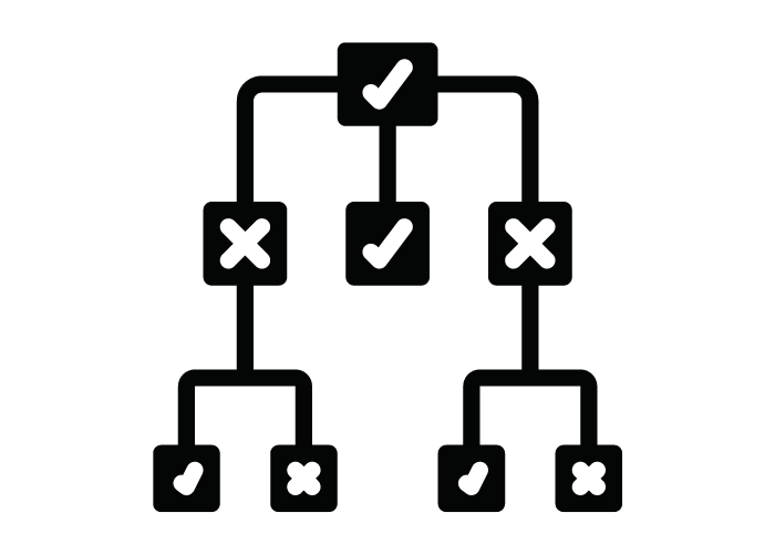 Decision tree. Image by Author
Here we can see we start with some initial condition, and depending on the outcome of that situation, we go into any three possible nodes. The outer nodes have another nested condition associated with them but the inner one is a final state.
One of the best things about DTs is that for our housing data example, we can build a tree that might say something like: "If the square footage is between 1000-2000 feet, then the value is $400,000". This is an oversimplification but you can use DTs for modeling regression examples as well as classification problems.
The reason this if/then structure is so important is that the tree itself actually becomes quite readable by a human. This is contrasted with ML models in the Deep Learning space, for example, where they are black boxes that we cannot usually understand. The explainability of DTs is one of the core reasons people use them in practice.
Decision Tree's Vs Linear Regression
Another important thing to point out about DTs, which is the key difference from linear models, is that DTs are commonly used to model non-linear relationships.
When dealing with problems where there are a lot of variables in play, decision trees are also very helpful at quickly identifying what the important variables are.
Now that we know the basics of decision trees (and if you still want to learn more about the more specific tree vernacular and such, check out this article), let's dive into some code examples and set up a tree.
Decision Tree's in Action 🌲🪓
For this example, we will be using the Iris dataset with the DecisionTree.jl package. We start off by loading in the dataset as follows:
using DecisionTree

features, labels = load_data("iris")
By default, the load_data function creates the features and labels variables to be of type any which is very computationally expensive. We can reduce this burden by converting the types explicitly to float and string, respectively:
features = float.(features)
labels   = string.(labels)
Next, we can call the build_tree function and pass in our labels and features:
model = build_tree(labels, features)
Now that we have our tree, we need to prune it to get some results.
model = prune_tree(model, 0.9)

# print of the tree with a depth of 6 nodes (optional)
print_tree(model, 6)
When we prune the tree, we can set the purity level to 90% in this case which means that we merge leaves that have 90% purity.
Purity in DTs is the idea that there is some data in each decision that falls into the wrong place. For example, we might only have 70% of the data we would expect to fall into a certain class fall into the class, which would give us 70% purity.
The print_tree function from above is a nice way of seeing what we have made so far:
Feature 4 < 0.8 ?
├─ Iris-setosa : 50/50
└─ Feature 4 < 1.75 ?
    ├─ Feature 3 < 4.95 ?
        ├─ Iris-versicolor : 47/48
        └─ Feature 4 < 1.55 ?
            ├─ Iris-virginica : 3/3
            └─ Feature 3 < 5.45 ?
                ├─ Iris-versicolor : 2/2
                └─ Iris-virginica : 1/1
    └─ Feature 3 < 4.85 ?
        ├─ Feature 1 < 5.95 ?
            ├─ Iris-versicolor : 1/1
            └─ Iris-virginica : 2/2
        └─ Iris-virginica : 43/43
This visualization shows us exactly what the tree is doing and how it is making these classification buckets. There are also more visualization tools like D3Trees.jl which would make this more interactive to view.
Now that we have the model, we can test it on a single data point:
julia> apply_tree(model, [5.9,3.0,5.1,1.9])
"Iris-virginica"
Or, we can make predictions on all of our data and look at the confusion matrix:
preds = apply_tree(model, features)

DecisionTree.confusion_matrix(labels, preds)

Classes:  ["Iris-setosa", "Iris-versicolor", "Iris-virginica"]
Matrix:   3×3 Matrix{Int64}:
 50   0   0
  0  50   0
  0   1  49

Accuracy: 0.9933333333333333
Kappa:    0.9899999999999998
3×3 Matrix{Int64}:
 50   0   0
  0  50   0
  0   1  49
As you can see, the accuracy of this model is actually quite good given the limited dataset and short training time.
This example should be enough to get you going on your DT journey, but if you need more help, check out this awesome video:
Wrapping up 👋
This post was a lightning-fast tour of some of the differences between Decision Trees and Linear Models as well as how to program them in Julia.
I hope you walk away from this with confidence that you can go and apply these tools in your own workflows!
If you enjoyed the article, please consider sharing it and you are always welcome to reach out to me on Twitter: https://twitter.com/OfficialLoganK
Happy programming!