
By Andrey Germanov
Julia is a general purpose programming language well suited for numerical analysis and computational science. Some consider it the future of machine learning and the most natural replacement for Python in this field.
This article introduces the Julia language and its ecosystem. You'll learn how to use it to solve a Titanic machine learning competition and submit it to the Kaggle.
You'll also learn how to deploy your machine learning model to production as a web service and create a web interface to send prediction requests to this service from a web browser.
By the end of the article, you will create a simple AI-powered web application that you can use as a template for creating more complex Julia ML solutions.
Here's what we'll cover:
- What You Should Know in Advance
- Why Use Julia for Machine Learning?
- How to Install Julia and Jupyter Notebook Support
- Julia Language Basics
- How to Visualize Data in Julia
- Overview of the Titanic Machine Learning Problem on Kaggle
- How to Prepare the Training Data for Machine Learning
- How to Train Our Machine Learning Model
- How to Make Predictions and Submit Them to Kaggle
- How to Deploy the Model to Production
- Conclusion
What You Should Know in Advance
This is not a book, but only an article. I won't cover everything and assume that you already have some base knowledge so you can get the most from reading it.
It is essential that you are familiar with Python machine learning and understand how to train machine learning models using Numpy, Pandas, SciKit-Learn and Matplotlib Python libraries.
Also, I assume that you are familiar with machine learning theory: types of machine learning problems like regression and classification, the concept and process of Supervised machine learning (fit/predict and evaluate quality using metrics) and common models used for it, including Random Forest Classifier, and it's implementation in SciKit-Learn Python library.
Additionally, it would be great if you've previously participated in Kaggle competitions, because to understand and run all code of this article you need to have an account on https://kaggle.com.
There are a lot of books already written, and many courses already released about the topics described above. In this article, my goal is to show you how to create, train, and deploy basic machine learning model using Julia, without diving to theoretical aspects of ML and AI.
Why Use Julia for Machine Learning?
For a long time, Python has been a standard for data science and machine learning because of it simplicity and great set of libraries and tools.
Among others there are great libraries like Numpy to help you do linear algebra with vectors and matrices, Pandas to manipulate datasets, Matplotlib for data visualizations, and Scikit-Learn that provides a uniform interface to work with well-known machine learning models.
Also, Jupyter Notebooks allow you to write and run Python code online right in a web browser. This creates a comfortable environment for data researchers to design and implement the whole machine learning cycle even if they are not very experienced in programming.
All this is good for research in laboratories, but at some point, you need to go to production. At this moment things change dramatically.
Python was created in the early nineties and was never supposed to be fast. It's kernel was never assumed to be used for new modern technologies like distributed computing.
That is why, to make complex ML tasks production-ready, you need to install a lot of third party dependencies. You'll also have to employ some tricks to speed Python code up. You can even rewrite or convert Python machine learning models before deploying them to production in faster languages like C++.
Well, Julia aimed to resolve these problems. This is what the authors wrote about why they created Julia:
We are greedy: we want more. We want a language that’s open source, with a liberal license. We want the speed of C with the dynamism of Ruby. We want a language that’s homoiconic, with true macros like Lisp, but with obvious, familiar mathematical notation like Matlab. We want something as usable for general programming as Python, as easy for statistics as R, as natural for string processing as Perl, as powerful for linear algebra as Matlab, as good at gluing programs together as the shell. Something that is dirt simple to learn, yet keeps the most serious hackers happy. We want it interactive and we want it compiled. Source: The Julia blog.
So, from an ML perspective, Julia got the best of both worlds. It was built to be as fast as C and as simple as Python. In addition, it has similar libraries that Python data scientists are used to incorporating into their work:
| Purpose | Python | Julia |
|---|---|---|
| Linear algebra | Numpy | Built in arrays, LinearAlgebra package |
| Work with datasets | Pandas | DataFrames.jl |
| Data visualization | Matplotlib | Plots.jl |
| Classic Machine learning | SciKit-Learn | MLJ.jl or ScikitLearn.jl |
| Neural Networks | TensorFlow or Pytorch | Flux.jl |
You can read more about why Julia is a great choice for machine learning here.
Furthermore, Julia has a module to support Jupyter Notebooks, so you can write Julia code there the same as with Python.
All this makes the Julia ready to do machine learning tasks, including Kaggle competitions, in the same environment as when using Python.
Now that you know why Julia is a great choice for ML, let's install this environment and introduce some Julia ML basics.
How to Install Julia and Jupyter Notebook Support
To install Julia, follow this link: https://julialang.org/downloads/. There, download the Julia package for your operating system and run it.
After successful installation, you will be able to run the julia command to enter the Julia REPL environment. Here, you can write and run Julia code. To exit from REPL, type the exit() command.
Also, you can write your code in any text editor and save to files with the .jl extension. Then you can run your Julia programs by this command:
julia <filename>.jl
In addition, you can use VSCode to develop in Julia. It has a great extension for this: https://www.julia-vscode.org/.
However, the best option to develop machine learning and data science solutions is using a Jupyter Notebook. So make sure that it's installed before continuing. Then, install the Jupyter support for Julia package using REPL:
- Enter REPL using the
juliacommand - Import
Pkgmodule like this:
using Pkg
- Then install the
IJuliapackage:
Pkg.add("IJulia")

* Exit REPL by using the `exit()` command

Then you can run Jupyter and create notebooks with Julia support. For your convenience, the next video shows how to install Julia and integrate it to Jupyter on macOS (assuming that Jupyter itself already installed).

%[https://youtu.be/rnJkT4G3-sE]

## Julia Language Basics

Julia has a simple syntax. If you're familiar with Python, then it will be easy to start writing in Julia. You can read more about basic Julia syntax in this [article](https://www.freecodecamp.org/news/learn-julia-programming-language/).

In this tutorial, I will only cover features that are required for machine learning and only the features which we'll use to solve the Titanic Kaggle competition. To learn more about each of these libraries and modules, I will provide useful links.

Create a new Jupyter Notebook to enter and run all the code samples below.

### Linear Algebra Features

Basic linear algebra features are already integrated into the Julia standard library. Each 1D array is a vector, and each 2D array works as a Numpy array by default. You do not need to include any additional packages for it.

For example, if you write and run this code:

```julia
A = [
    [1 2 3]
    [4 5 6]
    [7 8 9]
]
B = [
    [7 8 9]
    [4 5 6]
    [1 2 3]
]

A*B
It will do a matrix multiplication and will output the following result:
3×3 Matrix{Int64}:
 18   24   30
 54   69   84
 90  114  138
For additional features, you can import the LinearAlgebra module.
using LinearAlgebra
Then, you can use such functions as det, tr or inv with matrices to get their determinants, traces, or inverse matrices, respectively:
using LinearAlgebra

A = [
    [1 2 3]
    [4 5 6]
    [7 8 9]
]
println("Determinant: ",det(A))
println("Trace: ",tr(A))
println("Inverse: ")
inv(A)
You can learn more about the linear algebra features in the LinearAlgebra module documentation.
How to Work with Datasets in Julia
To work with datasets, you have to install an external Dataframes.jl module. In addition, to load and save datasets to CSV files, you have to add the CSV.jl module.
The Julia package manager is implemented as a Pkg module, so, you have to import it and then use the add method to install any required packages.
Run this in your Jupyter notebook to install these packages:
using Pkg
Pkg.add("DataFrames")
Pkg.add("CSV")
Then, you can import the installed modules to your program:
using DataFrames, CSV
The DataFrames module imports the DataFrame data type that you will use to construct datasets and manipulate data frame objects.
How to create a data frame
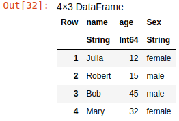
This is how you can create a data frame with two columns:
df = DataFrame(name=["Julia", "Robert", "Bob","Mary"], age=[12,15,45,32])
This code will create and output the following dataset:
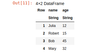 Persons data frame
How to select data from a data frame
To select data from a data frame, you can use the array syntax:
df[<rows>,<columns>]
You should specify the range of rows to select in <rows> and the range of columns to select in <columns>. You can use this to select first three rows and only the "age" column:
subs = df[1:3,"age"]
It's important to note that array numbering in Julia starts with 1, not with 0 as in most other languages. To select the first three rows and all columns, you can run this:
subs = df[1:3,:]
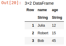 Select subset of rows from data frame
Also, to select a single column, you can use dot syntax:
names = df.name
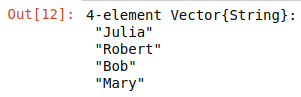 Names column
As you see, each column is a native Julia array (vector).
You can use conditions to specify row ranges. For example, you can use this code to select all persons from a dataset that are older than 15 years:
older = df[df.age .>15,:]
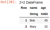 "older" data frame
This code will put all persons who are older than 15 years into the older data frame.
How to sort data in a data frame
To sort data in a data frame, you can use the sort function. This will sort the dataset by age in ascending order:
sort(df,"age")
 Sort data frame by age in ascending order
And this code will sort it in descending order:
sort(df,"age",rev=true)
 Sort data frame by age in descending order
How to add columns to a data frame
To add a new column, just use dot syntax:
df.sex = ["female","male","male","female"]
This added the sex column for persons to the data frame.
How to remove columns from a data frame
You can use the select function for more complex data extraction from frames. In particular, you can use it to extract all columns except the one(s) specified, which is equal to removing these columns:
new_df = select(df,Not("sex"))
This code returns a new data frame by selecting all columns from the original except sex.
How to group and summarize data in a data frame
You can use the groupby and combine functions to group data and show summary information for each group. The former groups data by specified field or fields and the latter adds summary columns to it, like number of rows in each group or average value of some column in the group.
The following code groups data by sex, calculates the number of rows in each group, and adds it as a "count" column:
group_df = groupby(df,"sex")
combine(group_df,nrow => "count")
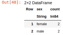 There are two females and two males in this dataset.
So, the first line of this code creates a GroupDataFrame object with rows, grouped by "sex". The second line creates the "count" column with count of items in each group. There are 2 females and 2 males in this dataset.
Also, you can use a custom function to calculate summary data. For example, you can use this code to add both row counts and average ages for each group:
combine(group_df,
    nrow => "count",
    "age" => ((rows) -> sum(rows)/length(rows)) => "Average Age"
)
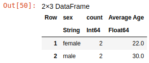
This code adds the "Average Age" column that is produced from the values of the "age" column by applying to it a custom anonymous function that calculates the average of values in this group.
This is just a small sample of all the possible manipulations that you can do with data using the DataFrames.jl library. You can read more about it in the documentation.
How to Visualize Data in Julia
Using Plots.jl, you can create a lot of different graphs to analyze your data, similar to Matplotlib or Seaborn in Python. To use it, you have to install the Plots package to your notebook and import it:
using Pkg
Pkg.add("Plots")
using Plots
Let me provide a few examples of graphs.
Line chart:
plot([1,2,3,4,5],[3,6,9,15,16],title="Basic line chart",label="Line")
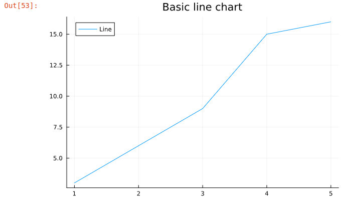 Basic line chart
Scatter plot:
plot([1,2,3,4,5],[3,6,9,15,16],title="Basic scatter plot",label="Data",seriestype="scatter")
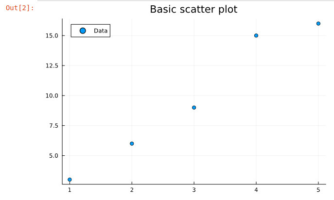 Basic scatter plot
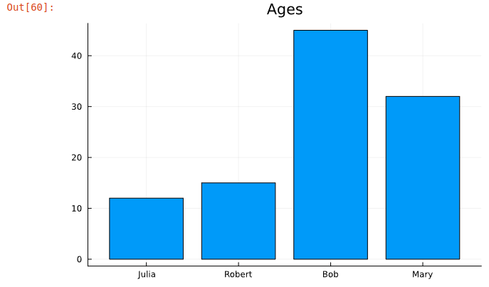
Bar chart:
The next code generates a bar chart from the df dataset that we created earlier.
plot(df.name,df.age,title="Ages",label=nothing,seriestype="bar")
 Bar chart
There's much more you can do using Plots.js. Read more about its features in the documentation.
After this short overview of basic data science features of Julia, it's time to create and train our first machine learning model and evaluate its quality in the competition.
Overview of the Titanic Machine Learning Problem on Kaggle
"Titanic - Machine Learning from Disaster" is one of the first educational machine learning problems that you might see in many books, articles, or courses.
In this task you are provided with a dataset of data about Titanic passengers. Each passenger data includes an ID, name, sex, ticket cost, ticket class, cabin number, port of embarkation and number of family members.
For passengers in this dataset, it's known whether they survived or not and the result is recorded in the "Survived" column. If the passenger survived, the value is 1, if not then 0.
Formally, this is called a labeled or training dataset. All data columns except one called the "feature matrix", and the "Survived" column called the "labels vector".
There is also the second dataset with the same data about other passengers but without the "Survived" column. In other words, this dataset contains only the features matrix, but does not have the labels vector. This is called the testing dataset.
The task is to train a machine learning model on the training dataset and use this model to predict the "Survived" column values in the testing dataset. In other words, its task is to predict the "labels vector" of the testing dataset based on its "features matrix".
The Kaggle competition is available here.
 The Titanic competition
Briefly read through the description, then open the "Evaluation" section to discover how Kaggle will evaluate the predictions that you submit.
How to Prepare the Training Data for Machine Learning
The "Data" tab on the Kaggle competition page contains training and testing datasets in train.csv and test.csv files, along with descriptions for each data column.
Create a new Jupyter notebook with a Julia back end and download these files to the same folder with your notebook.
Load train.csv to DataFrames using the CSV module:
# Add packages
using Pkg
Pkg.add("DataFrames")
Pkg.add("CSV")

# Import modules
using DataFrames, CSV

# Load training data to data frame
train_df = CSV.read("train.csv", DataFrame)
In case of errors, just make sure to check that the train.csv file exists in the folder where you run your notebook.
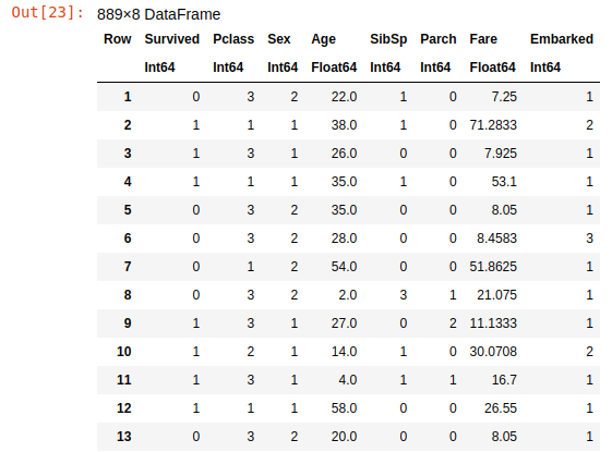
If there are no errors, it will show the first rows of the data:
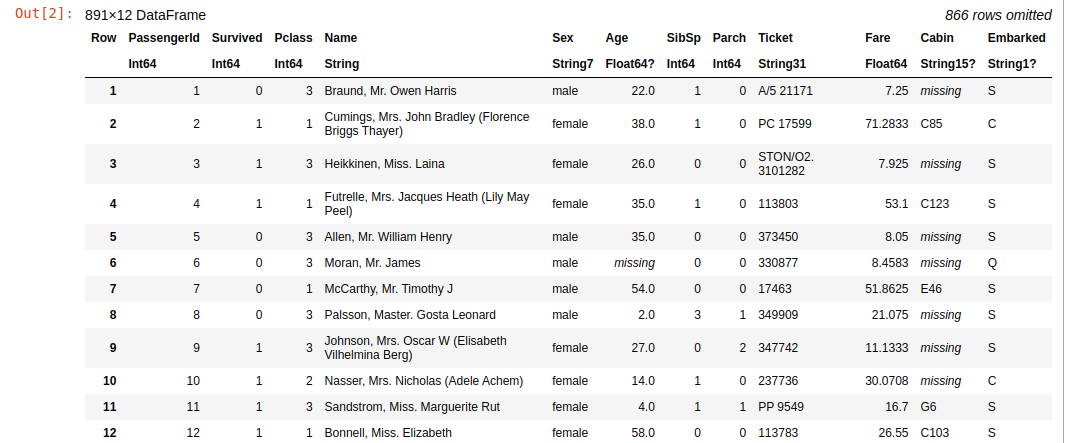 Training dataset
As you can see, this dataset has 891 rows and 12 columns. This is the basic data about passengers like "Name", "Sex" and "Age". In addition, we see the "Survived" column, with 0 if the passenger did not survive and 1 if they survived.
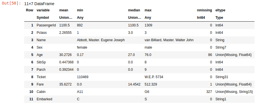
Let's see the summary information about this data using the describe function:
describe(train_df)
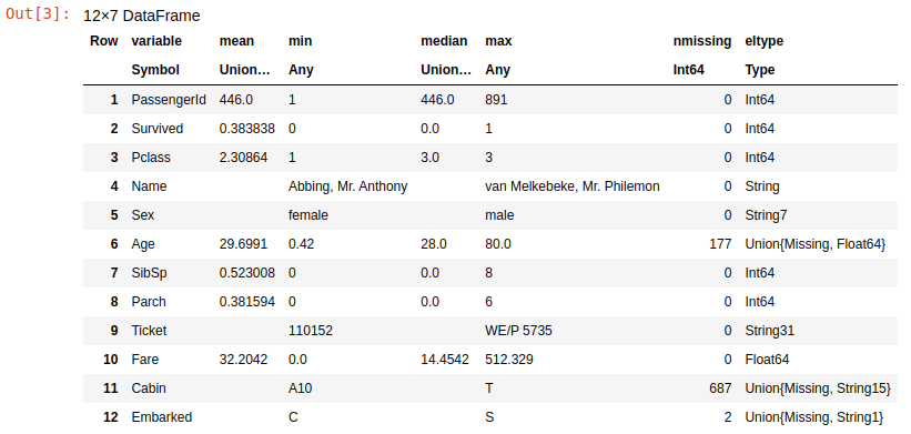 Training data summary
This summary table shows info about each column. It shows the min, max, mean and median of the data in each of them. The basic goal of the data preparation is to transform these columns to features matrice and labels vector.
The labels vector is ready – this is the "Survived" column with numeric values. All other columns form the features matrix, and not everything is ok with them.
Let's look at the nmissing and eltype for each column. The nmissing shows the number of missing values in the appropriate column, and the eltype shows the type of data values in them.
The matrix should contain only numbers, but there are many columns of "string" data type. Also, the matrix should not have missing values, but we have some missing values in Age, Cabin and Embarked columns. Let's fix all this.
How to Fix the Missing Values
As the previous table shows, the Age, Embarked and Cabin columns contain missing values. The Embarked has blanks in only 2 rows, so we will not lose too much data if just remove these rows.The DataFrames module has a handy dropmissing function you can use for this:
train_df = dropmissing(train_df,"Embarked")
This will remove all rows with missing values in the Embarked column.
The Age contains 177 missing values. It's not a good idea to remove these rows, because we will lose about 20% of data in the dataset. So, let's just fill it with something, for example with median value.
The median age is 28 as displayed in the description table. Let's use the replace function of DataFrames to replace the missing ages with a value of 28:
train_df.Age = replace(train_df.Age,missing=>28)
The Cabin column contains 687 missing values, which is more than 50% of the dataset. There are too few data in this column to be useful for predictions. Also, it's difficult to predict which data should be in these rows if more data is missing than exists. So, let's just drop this column using the select function:
train_df = select(train_df, Not("Cabin"))
Finally, all missing data in the dataset is fixed.
How to Fix Non-Numeric Data
As I explained before, all data should be encoded to numbers. But we have Name, PassengerId, Sex, Ticket and Embarked as strings.
The Name and the PassengerId values are unique for each passenger, so the ML model can't use them to split the data into categories or classify it. So, you can just remove these columns:
train_df = select(train_df,Not(["PassengerId","Name"]));
For other string columns, we need to encode all text values to numbers. To do that, need to discover all unique values of these columns. Let's start from the Embarked:
combine(groupby(train_df,"Embarked"),nrow=>"count")
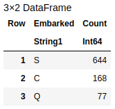 Embarked categories
This code grouped the dataset by the Embarked column and showed all possible values and their counts. So, here there are "S", "C" and "Q" values only. It's easy to encode them as S=1, C=2, and Q=3. You can do this simply with the following replace function:
train_df.Embarked = Int64.(replace(train_df.Embarked, "S" => 1, "C" => 2, "Q" => 3))
Also, this code converted the column from "String" to "Int64" data type.
Then, repeat the same for the Sex column:
combine(groupby(train_df,"Sex"),nrow=>"count")
 Sex categories
And replace female with 1 and male with 2.
train_df.Sex = Int64.(replace(train_df.Sex, "female" => 1, "male" => 2))
Now it's time to see the summary info for the Ticket column:
combine(groupby(train_df,"Ticket"),nrow=>"count")
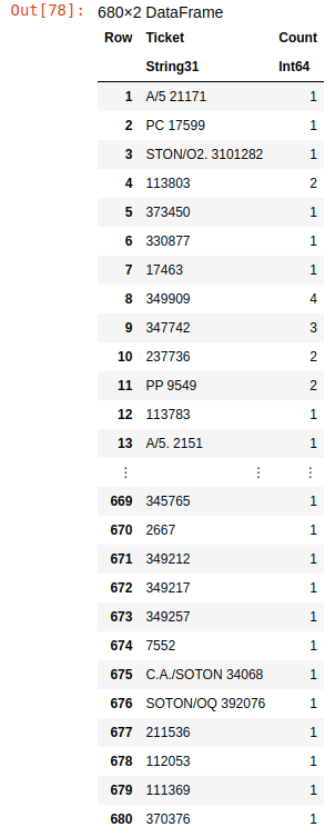 Ticket categories
Here we see that it has 680 different categories of tickets, which is more than 50% of the data. But we need to predict just two categories, either survived or not survived. We're not sure that this data can help the model make good predictions without additional processing to reduce the number of categories in this column.
Although this goes beyond our current basic model, as some additional practice, you can play around some more with the data in this column to improve prediction results. For example, you can try to find out how to group tickets to more general categories and encode these categories by unique numbers.
For now, let's just remove this column:
train_df = select(train_df,Not("Ticket"))
Now all the string data is categorized, and all values replaced with numbers. Let's describe the dataset again to ensure that all problems with the data have been resolved:
describe(train_df)
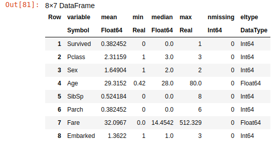 Fixed training dataset
You can see that all columns contain only numeric data and there are no missing values in them.
Visual Data Analysis
Now, we're ready to train a machine learning model on our dataset. Let's visualize this data to find some relationships in it.
using Plots

# Group dataset by "Survived" column
survived = combine(groupby(train_df,"Survived"), nrow => "Count")

# Display the data on bar chart
plot(survived.Survived, survived.Count, title="Survived Passengers", label=nothing, seriestype="bar", texts=survived.Count)

# Modify X axis to display text labels instead of numbers
xticks!([0:1:1;],["Not Survived","Survived"])
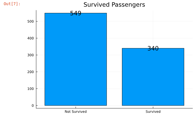
Here we see that 340 passengers survived. Now let's see how these passengers are distributed by sex.
# Group dataset by Sex column and show only rows where Survived=1
survived_by_sex = combine(groupby(train_df[train_df.Survived .== 1,:],"Sex"), nrow => "Count")

# Display the data on bar chart
plot(survived_by_sex.Sex, survived_by_sex.Count, title="Survived Passengers by Sex", label=nothing, seriestype="bar", texts=survived_by_sex.Count)

# Modify X axis to display text labels instead of numbers
xticks!([1:1:2;],["Female","Male"])

Interesting, there are two times as many females who survived than males in the training dataset. Now let's see the distribution of not survived passengers by ticket class.
# Group dataset by PClass column and show only rows where Survived=0
death_by_pclass = combine(groupby(train_df[train_df.Survived .== 0,:],"Pclass"), nrow => "Count")

# Display the data on bar chart
plot(death_by_pclass.Pclass, death_by_pclass.Count, title="Dead Passengers by Ticket class", label=nothing,
    seriestype="bar", texts=death_by_pclass.Count)

# Modify X axis to display text labels instead of numbers
xticks!([1:1:3;],["First","Second","Third"])
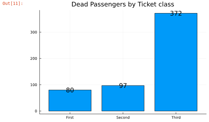
This clearly shows that first and second class passengers had more chance of survival than third class passangers.
Assuming that data in the training and the testing datasets are distributed randomly, it's highly likely that a machine learning model trained on this data should predict that women in first or second class had a much higher chance of survival than others.
Let's remember this finding to check this hypothesis at the end of the article, after we train and deploy the ML model.
Finally, let's see the cleaned training dataset again:
train_df
 The cleaned training set
Now it really looks like a matrix – or, to be more precise, like a system of algebraic linear equations written in matrix form. Data in matrix format is exactly what most machine learning algorithms expect to get as an input. Let's get started.
How to Train Our Machine Learning Model
For machine learning, we will use the SciKitLearn.jl library, which replicates the SciKit-Learn library for Python. It provides an interface for commonly used machine learning models like Logistic Regression, Decision Tree, or Random Forest.
SciKitLearn.jl is not a single package but a rich ecosystem with many packages, and you need to select which of them to install and import. You can find a list of supported models here. Some of them are built-in Julia models, others are imported from Python. Also, SciKitLearn.jl has a lot of tools to tune the learning process and evaluate results.
For this "Titanic" task, we will use the RandomForestClassifier model from the DecisionTree.jl package. Usually it works well for classification problems. Also, we will use the Cross Validation module to calculate accuracy of model predictions from the SciKitLearn.CrossValidation package.
You have to install and import these packages before using them:
Pkg.add("DecisionTree")
Pkg.add("SciKitLearn")
using DecisionTree, SciKitLearn.CrossValidation
Then we will implement the training process. First we need to split the training dataset into features matrix and labels vector. Then we need to create the RandomForestClassifier model and train it using this data. Finally, we will evaluate a prediction accuracy of this model using the cross_val_score function.
# Put "Survived" column to labels vector
y = train_df[:,"Survived"]
# Put all other columns to features matrix (important to convert to "Matrix" data type)
X = Matrix(train_df[:,Not(["Survived"])])

# Create Random Forest Classifier with 100 trees
model = RandomForestClassifier(n_trees=100)

# Train the model, using features matrix and labels vector
fit!(model,X,y)

# Evaluate the accuracy of predictions using Cross Validation
accuracy = minimum(cross_val_score(model, X, y, cv=5))
 The accuracy of trained ML model
The cross validation splits X and y arrays into 5 parts (folds) and returns the array of accuracies for each of these parts. Then the minimum function selects the worst accuracy from this array, which means that all others are better than the selected one.
Finally, the achieved accuracy is more than 0.78, which is 78% for our training data. It's not bad, but does not guarantee that on the testing dataset the result will be the same.
You can try to improve this value by selecting different models, or by tuning their hyperparameters.
For example, you can increase the number of trees (n_trees) from 100 to 1000 or reduce to 10 and see how it changes the accuracy. After achieving the best result, it's time to use it for predictions.
How to Make Predictions and Submit Them to Kaggle
Now, when the model is ready, it's time to apply it to data from the test.csv file which does not have the "survived" labels. First we need to load it and look at the summary table as we did for the training dataset:
test_df = CSV.read("test.csv",DataFrame)
describe(test_df)
 Testing dataset description
Here you can see the same problems with the data: missing values and string columns. You need to apply exactly the same transformations to this data as you did in the training dataset – except for removing rows, because the Kaggle requires that you do predictions for each row, so you can only fill in the missing values.
Fortunately, the Embarked column does not have missing values, so there is no need to fix it. This dataset has a single missing value in the Fare column, but we did not have any missing values there in the training set. It's not a big problem, as you can just replace this missing value by the median 14.4542.
But the first thing that we need to do is save the PassengerId column to a separate variable. It will be required later for the Kaggle submission.
PassengerId = test_df[:,"PassengerId"]
Then, apply all the required data fixing techniques:
# Repeat the same transformations as we did for training dataset
test_df = select(test_df,Not(["PassengerId","Name","Ticket","Cabin"]))
test_df.Age = replace(test_df.Age,missing=>28)
test_df.Embarked = replace(test_df.Embarked,"S" => 1, "C" => 2, "Q" => 3)
test_df.Embarked = convert.(Int64,test_df.Embarked)
test_df.Sex = replace(test_df.Sex,"female" => 1,"male" => 2)
test_df.Sex = convert.(Int64,test_df.Sex)

# In addition, replace missing value in 'Fare' field with median
test_df.Fare = replace(test_df.Fare,missing=>14.4542)
After the testing dataset is clean, you can use the trained model to make predictions:
Survived = predict(model, Matrix(test_df))
This code returns an array of predictions for each row of the testing dataset matrix and saves it to the Survived variable.
Now it's time to submit it to Kaggle. Before doing this, look again at the "Evaluation" tab on the Kaggle Titanic competition page to see the required submission format:
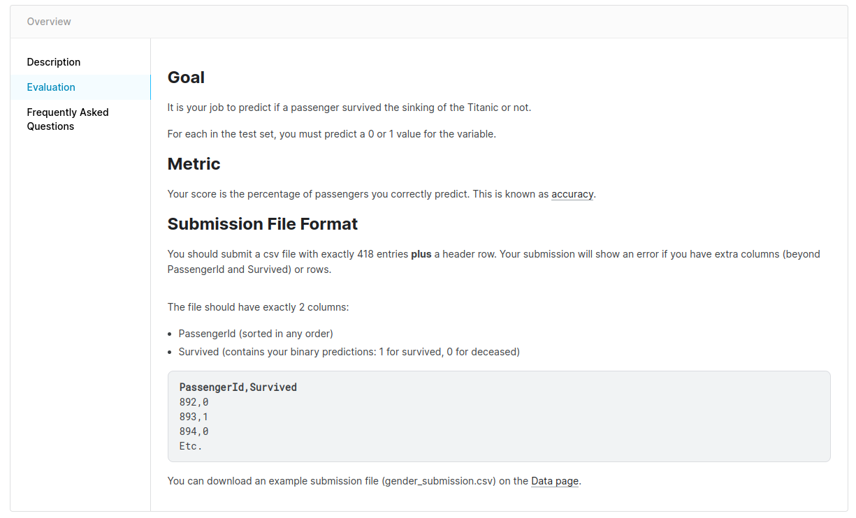 Kaggle submission rules description
The competition requires a CSV file with two columns: "PassengerId" and "Survived". You already have all this data. Let's create the data frame with these two columns and save it to a CSV file:
submit_df = DataFrame(PassengerId=PassengerId,Survived=Survived)
CSV.write("submission.csv",submit_df)
The first line of this code constructs the submit_df data frame with the PassengerId column that was saved previously and the Survived column with predictions for each passenger ID. The second line saves this submit_df to the submission.csv file. This is how the content of this file looks:
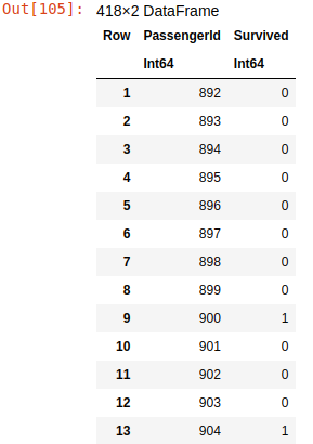 Data frame for Kaggle submission
Finally, go to the Kaggle competition page, press the "Submit Predictions" button, upload the submission.csv file, and see your result. When I did this, I received the following:
 Kaggle submission result
The prediction accuracy is 0.76555 which is more than 76% and is close to the accuracy that we got on the training dataset.
Not bad for the first time, but you can keep going: play with data, try different models, change their hyperparameters, surf the Internet for articles and Jupyter notebooks of other people who solved the Titanic competition before. I know that it's possible to achieve up to 98% accuracy using various tricks with models and data.
How to Deploy the Model to Production
It's fun to play around with machine learning on your computer, but it does not have much impact on real-world problems.
Usually, customers do not have Jupyter Notebooks and they do not train the models. They need to have a simple tool that will help them make decisions based on predictions from data that they have.
That is why the only really important thing is how your models work in production.
In this section, I will explain how to use Julia to create a web application that will load the machine learning model you trained to make predictions online in a web browser.
How to Export the Model to a File
First, you need to save the model from the notebook to a file. For this you can use the JLD2.jl module. This module used to serialize Julia objects to HDF5-compatible format (which is well known by Python data scientists) and save it to a file.
Install and load the package to the notebook:
Pkg.add("JLD2")
using JLD2
and then save the model variable to the titanic.jld2 file:
save_object("titanic.jld2", model)
We're done with our work with Jupyter Notebook now. You should write all the following code as a separate application.
Create a folder for a new application, like titanic for example, and copy the titanic.jld2 file to it.
Now you can create a text file titanic.jl which will contain the code of the web application that you will write soon. Use any text editor for this – VS Code with the Julia extension is a good choice. Enter the following code into titanic.jl:
using JLD2, DecisionTree
model = load_object("titanic2.jld2")
survived = predict(model,[1 2 35 0 2 144.5 1])
println(survived)
This code imports the required modules first. As you can see, just two modules are required to run the prediction process: JLD2 to load the model object, and DecisionTree to run the predict function for the RandomForestClassifier.
Then, the code loads the model from the file and it makes predictions for a single row of data. The columns in this row should go in the same order as passed from the dataset when we trained the model: Pclass, Sex, Age, SibSp, Parch, Fare and Embarked.
Finally, it prints the array of predictions. In this case, it will print the array with a single item, because only a single row of data was passed to the model for predictions.
You can run this code using the julia command:
julia titanic.jl
If everything worked ok, it should print [0] or [1] to the console depending on the prediction result. If you receive errors, then you might need to install the JLD2 and DecisionTree packages using the Julia REPL environment, as you did it in the Jupyter notebook.
Now, let's refactor this code to a function that will receive the row of data and return a survival prediction (either 0 or 1):
using JLD2, DecisionTree

# Returns 1 if a passenger with
# specified 'data' survived or 0 if not
function isSurvived(data)
    model = load_object("titanic2.jld2")
    survived = predict(model,data)
    return survived[1]
end
How to Create the Front End
The next step is to create a web interface that will be used to collect the data for this function. This will look like this:
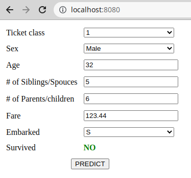 Web application user interface
With this interface, the user can enter the data about a passenger, then press the "PREDICT" button and discover whether the passenger with this data could survive on the Titanic or not. This is the HTML code for this web page:
<!DOCTYPE html>
<html lang="en">
<head>
    <meta charset="UTF-8">
    <meta http-equiv="X-UA-Compatible" content="IE=edge">
    <meta name="viewport" content="width=device-width, initial-scale=1.0">
    <title>Titanic</title>
</head>
<body>
    <table>
        <tbody>
            <tr>
                <td>Ticket class</td>
                <td>
                    <select id="pclass">
                        <option value="1">1</option>
                        <option value="2">2</option>
                        <option value="3">3</option>
                    </select>
                </td>
            </tr>
            <tr>
                <td>Sex</td>
                <td>
                    <select id="sex">
                        <option value="1">Female</option>
                        <option value="2">Male</option>
                    </select>
                </td>
            </tr>
            <tr>
                <td>Age</td>
                <td>
                    <input id="age" type="number"/>
                </td>
            </tr>
            <tr>
                <td># of Siblings/Spouces</td>
                <td>
                    <input id="sibsp" type="number"/>
                </td>
            </tr>
            <tr>
                <td># of Parents/children</td>
                <td>
                    <input id="parch" type="number"/>
                </td>
            </tr>
            <tr>
                <td>Fare</td>
                <td>
                    <input id="fare"/>
                </td>
            </tr>
            <tr>
                <td>Embarked</td>
                <td>
                    <select id="embarked">
                        <option value="1">S</option>
                        <option value="2">C</option>
                        <option value="3">Q</option>
                    </select>
                </td>
            </tr>
            <tr>
                <td>Survived</td>
                <td id="survived"></td>
            </tr>
            <tr>
                <td colspan="2">
                    <div>
                        <button id="submit" type="button">PREDICT</button>
                    </div>
                </td>
            </tr>
        </tbody>
    </table>
    <script>
        document.getElementById("survived").innerHTML = "";
        document.getElementById("submit").addEventListener("click",async() => {
            response = await fetch("http://localhost:8080",{
                method:"POST",
                body: JSON.stringify({
                    "pclass":parseInt(document.getElementById("pclass").value),
                    "sex":parseInt(document.getElementById("sex").value),
                    "age":parseFloat(document.getElementById("age").value),
                    "sibsp":parseInt(document.getElementById("sibsp").value),
                    "parch":parseInt(document.getElementById("parch").value),
                    "fare":parseFloat(document.getElementById("fare").value),
                    "embarked":parseInt(document.getElementById("embarked").value),
                })
            });
            const survivedCode =  parseInt(await response.text());
            document.getElementById("survived").innerHTML = survivedCode ? "YES" : "NO"
        })
    </script>
    <style>
        input,select {
            width:100%;
        }
        td {
            padding:5px;
        }
        td > div {
            text-align: center;
        }
        #survived {
            font-weight: bold;
            color:green;
        }
    </style>
</body>
</html>
Create an index.html file in the same folder and copy this code to it. The HTML part of the file contains a simple form with all data fields. As you can see, all values are encoded to the same numbers as we did with data in training and test datasets.
Then, the JavaScript part of this code defines the handler of the "PREDICT" button. When the user clicks on it, the script collects all entered data and saves it as a JSON string. Then it makes an AJAX request to the web service running on port 8080 of the localhost (which we have not created yet) and sends this JSON to the web service.
So, the web service should be able to receive HTTP POST requests with JSON body in the following format:
{
     "pclass": 1,
        "sex": 1,
        "age": 32,
      "sibsp": 5,
      "parch": 6,
       "fare": 123.44,
   "embarked": 1
}
How to Create the Back End
Now it's time to modify the julia.jl file to make it work as a web server that can display the index.html page, receive POST requests from it, parse the body of this request to JSON, make predictions based on this JSON data, and return this prediction to the web page.
Creating a web server on Julia is the same as on Python, Go, or Node.js. By using the HTTP.jl package, you can create and run a web server with a single line of code:
using HTTP

HTTP.serve(handler,8080)

function handler(req)
    # handle HTTP request
end
The HTTP.serve function runs the web server on the specified port. Each time when the web server receives a client request, it calls the specified handler function and sends an HTTP request object to it as a req argument.
The function should read this request, process it, and write a response to the calling client.
The req.url field contains the URL of the received request. The req.method field contains the request method, like GET or POST. The req.body field contains the POST body of the request in binary format. The HTTP request object contains a lot of other information. All this you can find in the HTTP.jl documentation.
Our web application will only check the request method. If the received request is a POST request, it will parse req.body to the JSON object and send the data from this object to the isSurvived function to make a prediction and return it to the client browser.
For all other request types, it will just return the content of the index.html file, to display the web interface.
This is how the whole source code of the titanic.jl web service looks:
using JLD2, DecisionTree

# Returns 1 if a passenger with
# specified 'data' survived or 0 if not
function isSurvived(data)
    model = load_object("titanic.jld2")
    survived = predict(model,data)
    return survived[1]
end

using HTTP,JSON3

function handle(req)
    if req.method == "POST"
        form = JSON3.read(String(req.body))
        survived = isSurvived([
            form.pclass
            form.sex
            form.age
            form.sibsp
            form.parch
            form.fare
            form.embarked
        ])
        return HTTP.Response(200,"$survived")
    end
    return HTTP.Response(200,read("./index.html"))
end

HTTP.serve(handle, 8080)
Before running it, you need to install the HTTP.jl package by running Pkg.add("HTTP") in the julia REPL environment.
The web service code goes right after the isSurvived function. First, the required modules are imported: HTTP to create a web server and JSON3 to parse JSON from request body.
Then, the handler function gets defined. The function checks the request method of the received requests and if it's equal to POST, it converts the stringified JSON body of this request to the form object. Then, using fields of this object, the isSurvived function gets called.
It's important to put array items in the correct order here.
Finally, the prediction result is returned to the client using the HTTP.Response function.
For all other request types, the function returns the body of the index.html file in the HTTP.Response(200,read("./index.html")) line.
Finally, the HTTP.serve function starts a web server on port 8080 that waits for the HTTP requests and handles them using the handle function, as defined above.
Now you can run this by typing julia titanic.jl in the terminal or by pressing Ctrl+F5 in VSCode. Then you can access the web interface from a web browser on http://localhost:8080 and play with the service by entering data in the form, pressing the PREDICT button, and seeing either YES or NO on the Survived line depending on the prediction result.
You can check the hypothesis which we made from bar charts: the women in 1st or 2nd class have more chance of survival than others.
Conclusion
In this article, I introduced you to the Julia programming language along with its ecosystem and explained why it's so great for machine learning.
I showed you how to set up a comfortable development environment and gave a brief overview of the common Julia modules used for data science.
Then I guided you through the process of training the machine learning model for the Titanic competition and showed you how to make predictions and submit them to the Kaggle platform for scoring.
Finally, I showed how to export this model to an external application, create the web service with this model and the web interface to enter data to the form, and predict whether the human with this data could survive on the Titanic or not.
For all topics that explained briefly, I provided the links with more thorough documentation. In addition, I would highly recommend reading this Julia Data Science online book and studying the great set of machine learning examples in Julia Academy Data Science GitHub repository.
See the source code of this article including the Jupyter Notebook and the web service in this repository.
Have a fun coding and never stop learning!
You can find me on LinkedIn, Twitter, and Facebook to know first about new articles like this one and other software development news.