

Discrete mathematics is an area of math based on the study of formal structures whose nature is fundamentally separate and distinct.
This means it focuses on integers and natural sets of numbers, shapes, and other objects that you can count finitely or distinguish from one another. It models reality in a manner specifically suited to certain real-world applications.
From industry and logistics to computer science and telecommunications, having a quantized representation of everything around us has led to magnificent advances in our understanding and control of the physical world.
It's important to have at least a rough idea of the main distinctions between discreteness and continuity to address graph theory. But these aren't very well-known concepts to people outside the world of mathematics.
At first, continuous math is the one predominantly taught in the education system due to its versatility, usefulness, and practicality in most areas.
It’s based on the analysis of real numbers and functions that encapsulate mappings between these quantities, along with the notion of the infinitesimal change of a variable. This results in a series of tools like limits or derivatives that constitute calculus.
On the other hand, the discrete paradigm is more straightforward and intuitive, with the exception of a few cases. And its finiteness is given by the primordial element constituting it – sets.
Among the most notorious use areas are those whose main components imply algorithms and data structures. Although the use cases of math are not what most people think they are.
In the real world, we don’t often face problems in the same way as in the education system. Indeed, discrete ways of approaching riddles and modeling the input data we need to come up with a solution are more usual than continuous ones, especially regarding system optimization issues.
For this reason, we should reconsider the role of this way of doing mathematics since it involves the development of critical/computational thinking. This is crucial for the current era in which we are surrounded by technology. It also involves the improvement of problem-solving skills, making it possible for us to face any new challenges.
By doing so, we can see how relevant it is to apply a solid mathematical foundation to common global threats that are increasing daily, like misinformation, lack of fluency in handling technology, geopolitical instability, and even climate change.
Notwithstanding the apparent remoteness between the latter issue and graph theory itself, we should think about the way we live and the system by which our civilization is maintained as we know it.
Goals of this Article
This article aims to explain graph theory, one of the most significant components of all discrete mathematics, in an intuitive, simple, and visual way. I'll also try to guide its use towards the development of new disruptive techniques applicable in areas such as environmental care, necessary to preserve and regenerate our nature.
Effectively achieving this will not only foster curiosity or inspire readers who may intend to continue learning, but will also contribute to a further rising in society’s awareness about sustainability issues. This will increase the likelihood that in the future, the problems that scientists predict to be threatening to our existence and the existence of life on the planet will be curbed, thanks to scientific knowledge and specifically the contribution of graph theory.
Still, given its broad scope, it will be impossible to explain graph theory entirely in this article. So, I'll focus on the visual side of any explanation over the formal one since you can easily consult that in any textbook. That will also provide a different point of view from certain definitions.
Also, it's essential that we treat the idea of a graph as comprehensively as possible. We'll focus on its history, representation, and most descriptive properties instead of advanced concepts like singular cycles. This will help you grasp the kernel of graph theory and prepare you to learn these advanced concepts more easily.
Here's what we'll cover:
- Basic Elements of Graph Theory
- History of Graph Theory
- Definition of a Graph
- Representations of Graphs
- Properties of Graphs
- Algorithms and Graph Theory
- Why Are Graphs Important in Achieving Sustainability?
- Conclusion
Basic Elements of Graph Theory
Whether you are new to Graph Theory or already know something about it, reviewing the basics is always worthwhile.
First, let’s introduce the idea of a “graph” with a usual representation you may have seen:
 Example of an arbitrary graph
Above, you have a graph where we can see, at the most fundamental level, two different building blocks: vertices (shown as circles) and edges (shown as lines connecting circles).
You can create a structure with those elements that can encapsulate the functioning of many systems present in our life that we don’t even realize.
But, most surprising of all is that graph theory as a whole is derived from such a simple concept as objects linked to each other.
History of Graph Theory
To understand the origin of this idea, we have to look back to the 18th century, when Leonhard Euler solved the famous Seven Bridges of Königsberg problem.
By that time, the city was crossed by the Pregel river, generating four pieces of land interconnected with seven bridges, as seen below:
 _Image extracted from [here](https://en.wikipedia.org/wiki/File:Konigsbergbridges.png" rel="noopener)
The task consisted of finding a path that crosses all bridges without passing by the same bridge twice, starting and ending at the same point.
At first, with so few bridges, it may be easy to find a brute force solution by trying combinations of paths. But, since we don’t know if a feasible solution exists, it’s helpful to formalize the problem elements and correctly prove its solvability before starting any process.
Also, if the number of bridges increases, it will become much more complex to solve, as the combinations increase remarkably fast.
 Königsberg problem displayed as a graph
As seen above, Euler represented land areas with graph vertices (also called nodes) and bridges with edges, concluding that it was impossible to have such a traversal through the graph.
Briefly, if we look at the number of edges incident to each vertex, we will see that every value is odd for every node, meaning that the graph does not have an eulerian cycle. This means that it’s not an eulerian graph, and we can’t positively prove the problem.
Nevertheless, this approach represented a breakthrough in the mathematical conception of various questions that were yet unsolvable. Euler’s contributions to the elaboration of this theory, which has been perfected and broadened over the years, made him one of the most influential mathematicians of his time.
Definition of a Graph
Now that you know what a graph looks like drawn on a diagram, let’s review the official formal definition:
A graph G is a pair of sets (V, E) where V is a non-zero set containing the graph’s vertices and E is a set made of element pairs belonging to V.
 Formal definition of a graph with its corresponding sets
Above, we represented the two main components of a graph in two corresponding sets, one for vertices V and another for edges E. So, our graph G is ultimately an ordered pair of these sets. But before we continue, we must look inside those sets to see what they look like and understand why.
On the one hand, V is a collection of items v in which each element contains the necessary data to define a vertex. Abstractly they are called with the letter v and a numerical subindex.
But in practice, they can be complex objects holding parameters, profiles, and so on.
On the other hand, the set of edges E is a little more complicated to define since it needs to determine the connections between vertices. In this case, the elements are unordered pairs of vertices from set V such that each pair is of the form {x, y}.
 Both formal and graphical representations of a graph
To familiarize yourself with these structures above, you have an arbitrary, fully defined graph with its respective sets. In V, you can see all the vertices numbered from 1 to 5 and placed in the upper diagram in a specific distribution, but you can arrange them according to your needs.
Meanwhile, in E, you can observe all the edges (lines) establishing an interconnection link between vertices.
The appropriate terminology to address this link is the following: for instance, if we have the edge {v1, v4}, we call it incident to v1 and v4. Also, those vertices are denoted to be adjacent since an edge links them.
As you may notice, there isn’t an edge {v4, v1} in E. But to find an explanation for this phenomenon, we have to introduce the main distinction that generates two classes of graphs.
The first one (undirected), to which the above examples belong, includes all graphs whose edges can be traversed in both directions. This makes them unordered pairs of vertices.
On the other hand, we can have a graph in which all its edges can only be traversed in one direction, that is, from one vertex to another exclusively. Thus, its vertex pairs on E set must be ordered, meaning that going from v1 to v4 is not the same as going from v4 to v1. This second class is known as a directed graph.
 Example of a directed graph.
Before learning how to represent a graph computationally to perform operations on it, you need to understand the vertex degree concept.
In undirected graphs, the degree of a vertex refers to the number of edges incident to it, considering that self-connecting edges (loops) count as 2 in the total score.
By contrast, in directed graphs, we have in-degree and out-degree values for each vertex, representing the number of incoming and outcoming edges, respectively.
Representations of Graphs
 The 2 most popular ways to computationally store a graph
Sometimes, the most intuitive solution for a problem is not always the most efficient in computer science. In this context, it generates different ways of representing a graph according to a problem’s nature.
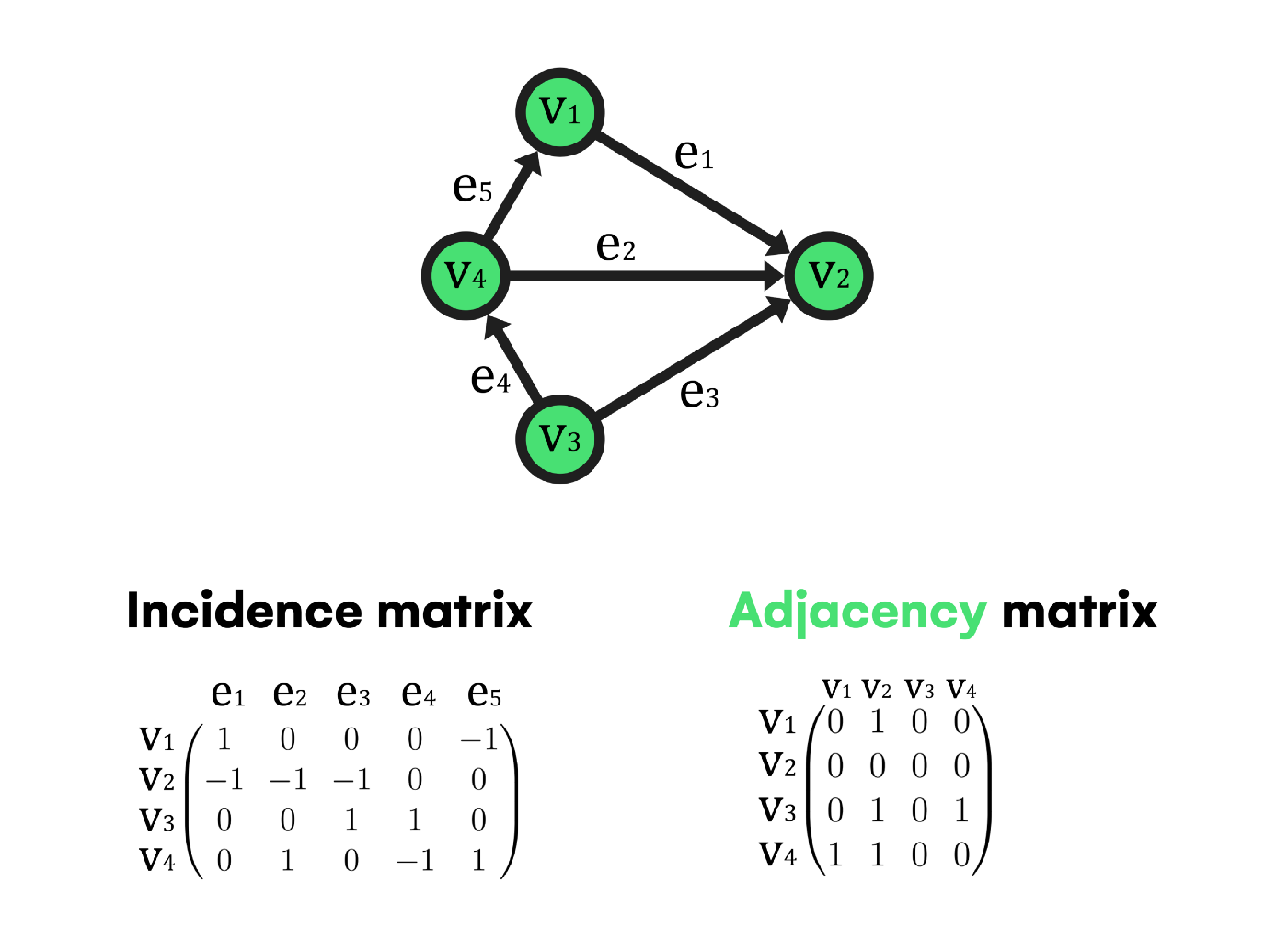
What is an Adjacency Matrix?
An adjacency matrix is one of the most popular methods to store a graph on a computer. But its major drawback is unused memory consumption.
For directed graphs like the one above, there is a matrix size |V|x|V| (being |V| the cardinality of the vertices set, thus the number of vertices on the graph) where each element can be a 0 if there is no connection between vertices or a 1 if the row element links the column one by an outgoing edge. Also, if the graph is weighted, the 1 value is substituted with the weight parameter associated with each edge when necessary.
However, if the graph is undirected, the same criteria apply with the difference that no distinction is made between outgoing and incoming edges this time. So there will be a 1 value if an edge exists between the row and column elements.
 Adjacency matrix element definition for each type of graph.
What is an Incidence Matrix?
Similar to the previous method, there is a matrix size |V|x|E| in which the same rules are fulfilled. The difference is that if an edge e is incoming to a vertex v, the corresponding element will be a -1 instead of 0.
How to Use Adjacency Lists
When using matrices, if the graph has many vertices but few edges (a sparse graph), the matrix will contain a high number of zeroes. This wastes a lot of memory and makes the representation inefficient in terms of space.
To solve this issue, adjacency lists appeared as an alternative replacing matrices with a combination of different data structures – arrays, and linked lists.
The kernel of this method is an array containing all the graph’s nodes. Each array element will have a linked list holding each leading node’s neighbor vertices (adjacent vertices). In the case of directed graphs, only the neighbor elements connected by an outgoing edge from the lead node will be inside the linked list.
 Example of a graph depicted as an adjacency list
So if we have a dense graph with a high number of edges, we should store it in matrix form. This has the advantage of O(1) time complexity when checking vertex connection and matrix symmetry along the main diagonal in undirected graphs.
But, if our graph is sparse, the low density of edges make an adjacency list the best choice to depict it computationally.
Properties of Graphs
Like any other mathematical object, graphs have specific properties that make them unique and functional for their purposes. Some have to do with their composition, others with topology, and even accessibility.
Undoubtedly, the most relevant properties concern traversals, since they allow us to model and optimize real-world scenarios.
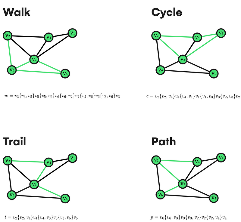
What is a graph traversal?
First, we need a starting node v1 and an ending node v2 to traverse a graph. Then, we can define a walk from v1 to v2 as an alternate sequence of vertices and edges. There, we can go through these elements as much as we need, and there is always an edge after a vertex (except the last one).
In the case of v1 being equal to v2, the walk would be closed.
Still, we can add repetition restrictions. So if we want a walk in which no edge is repeated, it’s renamed as “trail”. Consequently, if the trail is closed, it would be denoted as “circuit”.
The same happens if we restrict vertex repetition – the walk renames to “path,” and a closed path is known as a “cycle”.
 Formal and graphical examples of network traversal types.
This traversing ability comes along with an interesting property valid for all existing undirected/directed graphs. It’s formalized as follows:
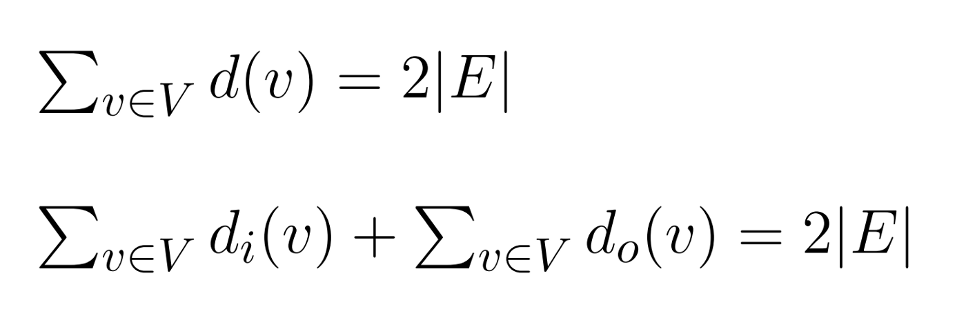 Formalization of the degree sum property.
This establishes that the sum of all vertex degrees equals two times the cardinality of the edge set in an undirected graph. If directed, the sum breaks into two terms, each referring to each node in and out-degree.
This is fairly straightforward to prove, because every time you add an edge to a graph, you need two vertices to build the pair of elements stored on E. So if you add a loop (edge linking a node with itself), you anyways need to define a pair of elements from V, regardless of whether they are the same.
This characteristic supports us when solving questions like:
Given a 6-regular graph (with all its vertex degrees set to 6) of n vertices, how many edges will it have?
As its resolution is immediate, going deeper when thinking about similar questions improves your understanding of its nature and why it's that way.
What is Connectivity?
Now, let’s move on to the properties related to the graph’s linking capability. Starting with an undirected graph, we can assure that a vertex v reaches u if there's a path from v to u. Also, we can look at the whole graph and define it as connected if every pair of vertices in it is indeed connected.
Being connected is often associated with the uniqueness of its components. That is, if we end up with a disconnected graph, its number of components will always be greater than 1.
You can imagine a component as a zone of the graph isolated and disconnected from the rest of the vertices. And this, if we consider a graph, will be connected and will only have one connected component as if it were a connected graph.
 Example of a 2 component made graph.
In contrast, when dealing with directed graphs, two vertices u and v are said to be strongly connected if they can reach each other and weakly connected if they are connected on the underlying (all edges replaced by undirected ones) graph.
As you can imagine, these properties generate many possibilities and new characteristics to consider.
To briefly mention, we can take advantage of the discrete nature of graphs to remove nodes and edges from them. Therefore, concepts such as articulation points or bridges emerge as one of the simplest ways to study a graph’s weak points.
An articulation point is a vertex that, if we remove from the graph together with all its incident edges, the graph will increase its connected components.
Likewise, a bridge is just an edge meeting the same previous condition with the difference that no vertex is removed from the graph.
 Visual example of an articulation point and a bridge.
As an extension to the properties section, it’s worth mentioning some tools and characteristics of graphs that will help us recognize the key of the algorithms we will see later:
What are Subgraphs?
Their name is an appropriate indicator of what subgraphs are, since it is quite illustrative. A subgraph is a collection of vertices and edges that we can extract from an arbitrary graph G to form another graph, usually undersized.
Formally, a graph H is a subgraph of G if it’s formed by a subset of vertices of G and similarly a subset of edges of G, with every edge being a valid pair of nodes.
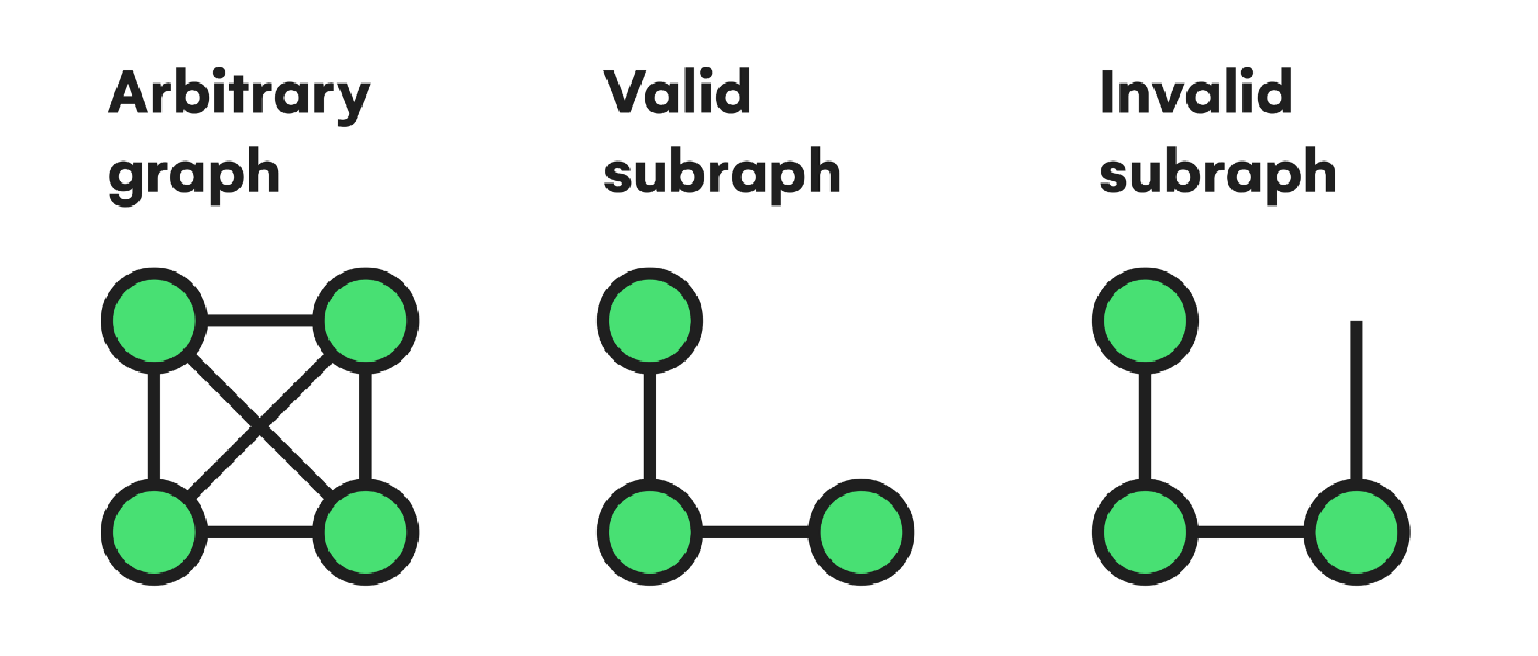 Example of a subgraph validity
The number of classifications and research we can perform about subgraphs makes it impossible to cover everything here. But the basis for further learning we'll start with the following ideas about its morphology, topology, and composition.
A subgraph H spans a graph G if both have the same vertices stored on V set. In this situation, subgraph H is known as a spanning subgraph.
 Example of a spanning subgraph.
Given a graph G, if we apply the vertex removal operation n times with n<|V|, the resulting graph will be an induced graph.
 Steps taken to reach an induced graph.
Topology doesn't just concern subgraphs. It's also mainly studied with general graphs. So reviewing some broad classifications and features will make graph theory more manageable.
A graph is said to be complete if it’s undirected, has no loops, and every pair of distinct nodes is connected with only one edge. Also, we can have an n-complete graph Kn depending on the number of vertices.
 Example of the first 5 complete graphs.
We should also talk about the area of graph coloring. A graph is bipartite when its nodes can be divided into two disjoint sets whose union results in the whole initial vertex set, with the condition that every edge has its extremes on both sets simultaneously. This allows for the possibility of coloring each vertex set with a different color.
Also, it can be a complete-bipartite graph if both sets are densely connected (every vertex of one set is connected with all vertices of the other collection).
 Some examples of arbitrary complete-bipartite graphs.
You might also need to represent a graph in a plane without any of its edges intersecting. Then, if possible, the graph will be planar. To better understand the state of this characteristic, we can use Kuratowski’s theorem. It involves advanced concepts like isomorphism and homomorphism concerning k5 complete and k3,3 complete bipartite graphs.
 Visual difference between planar and non-planar graphs.
What are Particular Cycles?
Finally, some graph features deserve special attention. For example, when it’s a matter of cycle finding, there's a deep relationship with vertex degrees, integral graph topology, and traversability.
To visualize this relationship, we'll return to the Königsberg problem. In it, we need to traverse all the graph’s edges without repeating any of them, starting and finishing in the same vertex.
Since graphs were new then, Euler developed a solution by defining a unique type of cycle only found in graphs meeting precise conditions – like the degree of all their nodes being even.
These cycles were named Eulerian after their creator, and every graph that has one is also called an Eulerian graph.
There are also Eulerian Paths. These remove the condition of having to start and end on the same vertex and require the graph to have exactly two odd-degree nodes, which will be the path extremes.
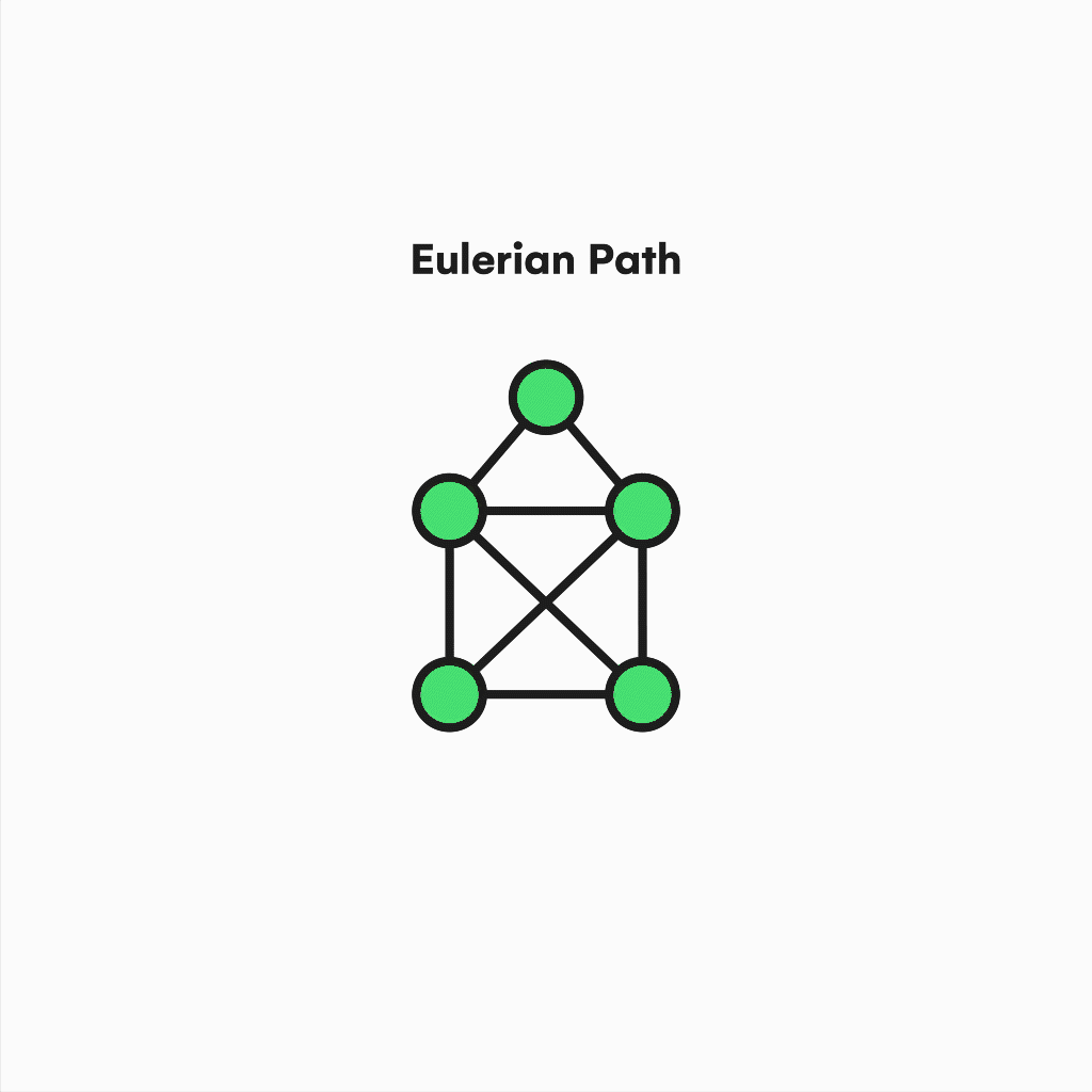 Visualization of an eulerian path.
Also, suppose we focus on contemporary issues like the traveling salesman problem (TSP), an NP-Hard problem mainly used by delivery and logistic companies.
In that case, we will realize the relevance of the hamiltonian cycles and paths to support practical solutions to similar questions. Similar to the eulerianity, a graph is Hamiltonian if it contains a cycle in which every vertex is used instead of edges.
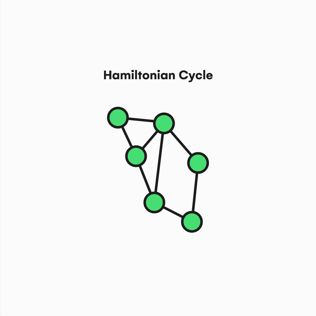 Visualization of a hamiltonian cycle.
These latter properties become challenging to deal with, given the complexity of the problems involved. Although, knowing the critical foundation supporting everything around them allows us to continue exploring with reasonable confidence.
Algorithms and Graph Theory
Once you have a solid grasp of graph theory, its elements, attributes, and tools, we should also review some basic algorithms comprising the principles of almost all other graph processes. Then we can move on to graph theory's use in climate preservation projects.
Breadth-first search algorithm
Here, we will only consider 3 algorithms since there are many types and very specialized ones for determined tasks.
To start with something simple and intuitive, we will unscramble Breadth-First Search. It's a graph traversal algorithm used to go through a graph in a breadthward motion.
In simple terms, it starts at an arbitrary vertex and iteratively visits its adjacent vertices, repeating this step until there are no more unvisited ones.
This behavior serves as the shortest path finder across all graph nodes, although you can stop the execution when a particular vertex is visited.
 Representation of breadth-first search algorithm
Depth-first search algorithm
The second algorithm is a variant of the previous one, known as Depth First Search. Its goal is similar but is also useful when detecting cycles, connected components, topological sorting, or checking for graph bipartitions.
But the way it works differs in some aspects, like the precedence of the depth over breadth – that is, not all neighboring nodes are visited in each step. Instead, one of them is chosen for further deepening, and the process is repeated until the path reaches a dead end and recursively goes back to the starting node, visiting every vertex.
 Representation of depth-first search algorithm
Dijkstra's Shortest-Path algorithm
Finally, the last one we will treat is Dijkstra’s algorithm, the most widespread Single Source Shortest Path problem solver ever created.
It’s designed to operate in weighted graphs with non-negative weights, and tries to find the most efficient route between 2 selected nodes.
Compared to the previous algorithms, that change increases the number of steps before completion. However, the key idea behind it is straightforward:
 Example Graph used to explain Dijkstra's algorithm
As you can see in the above example, if we want to go from v1 to v2, we can select the edge between them and arrive at our destination after traversing six distance units.
On the other hand, if we choose to go through the v3 or v4 paths, we would be walking seven units. So we need to make a decision on whether or not to take a particular path.
On large graphs, the algorithm calculates the provisional shortest paths along every single node. It then updates these values and minimizes “distance” (given by weights) by a complete graph traversal, as you can see in this animation.
Why Are Graphs Important in Achieving Sustainability?
At this point, you may realize that Graph Theory is valuable because it can encapsulate and abstractly model problems of a nuanced nature. Especially those problems whose origin stems from society’s need to pursue a degree of globalization that brings a standard of wellness to everyone’s lives.
Yet many of us are unaware that the comfort we currently enjoy brought about by advances in communications, transport, nutrition, and entertainment requires the coordinated operation of complex systems to be in place.
So the overpopulation experienced since the twentieth century causes these systems to be so massive that they entail a severe environmental impact based on CO2 emissions and the systematic dumping of waste into natural environments.
Graphs can help with transportation of goods
In this context, everything involving the transport of goods and logistics contributes a significant amount of CO2 to the atmosphere. Here is where using graphs has a clear benefit for the environment. They can find optimal paths between cities or world locations, reducing the emissions of the vehicles engaged in such transport.
For example, you can experiment with Google Maps by tracing routes between distant places. You will notice it can automatically choose an appropriate route, minimizing the corresponding environmental cost.
Google Maps is working is based on Single Source Shortest Path algorithms like Dijkstra or advanced ones such as A-star. A-star is a heuristic variant of Dijkstra. These are used in combination with other state-of-the-art graph mechanics used to add certain constraints to algorithms.
Graphs can help with waste management
Graphs also have a place in the global industry by simulating or directly managing networks, manufacturing processes, and schedules. They can potentially reduce the amount of incorrectly handled/wasted energy and resources.
It’s also worth mentioning the numerous possibilities that graphs have to offer when we deal with the problem of excessive waste accumulation.
Nowadays, it's widely believed that plants and trees are the major contributors to oxygen in our atmosphere thanks to photosynthesis. But we have to account that between 50% and 85% of the oxygen released into the atmosphere each year is produced under the sea.
Ironically, data on waste thrown into the ocean are constantly increasing as the consumer society advances on time, causing a dramatic impact on the actual lungs of our planet, as well as on the animal species it shelters.
To avoid having to decide where to dump our garbage, we can use graph theory to generate simulations of molecular physical systems, atomic structures, and chemical reactions to develop new recyclable or biodegradable materials. These would reduce the environmental impact of the products we use.
Also, these simulations have the potential to be useful in biology, where deciphering the ultimate workings of DNA can lead to better food quality, as well as more efficient mass-production methods.
Graphs can help with machine learning and AI
Finally, the most well-known application of graphs is in the field of machine learning.
Despite all the other significant uses for graphs in computer science (like communication networks, distributed systems, or data structures), machine learning has shown us with its exponential evolution over the last decade that it is a highly promising technology when tackling climate change.
Simply put, machine learning is a subset of artificial intelligence that focuses on enabling machines to learn and detect patterns on large datasets. Sometimes, this learning is inspired by natural phenomena like synapses on human neurons, resulting in new techniques such as Artificial Neural Networks.
Regarding environmental care, the ability of these techniques to analyze large amounts of data makes it possible to measure our effect on the planet better.
As a real working example, Joinus4theplanet is an initiative focused on taking advantage of social media to raise awareness about the value of sustainability. It has developed a machine learning system able to perform waste sorting with the help of convolutional models designed to process multidimensional data in order to palliate the effects of incorrect recycling.
 Example of a social network is represented as a graph. Image from [Wikipedia.](https://en.wikipedia.org/wiki/File:SocialNetworkAnalysis.png" rel="noopener ugc nofollow)
Conclusion
If we want to maintain a considerable amount of progress inside our civilizations and provide a thriving future for the next generations, we have to consider graphs as an essential tool when rethinking the way our technological and economic systems work.