
By Bert Carremans
When applying one-hot encoding to words, we end up with sparse (containing many zeros) vectors of high dimensionality. On large data sets, this could cause performance issues.
Additionally, one-hot encoding does not take into account the semantics of the words. So words like airplane and aircraft are considered to be two different features while we know that they have a very similar meaning. Word embeddings address these two issues.
Word embeddings are dense vectors with much lower dimensionality. Secondly, the semantic relationships between words are reflected in the distance and direction of the vectors.
We will work with the TwitterAirlineSentiment data set on Kaggle. This data set contains roughly 15K tweets with 3 possible classes for the sentiment (positive, negative and neutral). In my previous post, we tried to classify the tweets by tokenizing the words and applying two classifiers. Let’s see if word embeddings can outperform that.
After reading this tutorial you will know how to compute task-specific word embeddings with the Embedding layer of Keras. Secondly, we will investigate whether word embeddings trained on a larger corpus can improve the accuracy of our model.
The structure of this tutorial is:
- Intuition behind word embeddings
- Project set-up
- Data preparation
- Keras and its Embedding layer
- Pre-trained word embeddings — GloVe
- Training word embeddings with more dimensions
Intuition behind word embeddings
Before we can use words in a classifier, we need to convert them into numbers. One way to do that is to simply map words to integers. Another way is to one-hot encode words. Each tweet could then be represented as a vector with a dimension equal to (a limited set of) the words in the corpus. The words occurring in the tweet have a value of 1 in the vector. All other vector values equal zero.
Word embeddings are computed differently. Each word is positioned into a multi-dimensional space. The number of dimensions in this space is chosen by the data scientist. You can experiment with different dimensions and see what provides the best result.
The vector values for a word represent its position in this embedding space. Synonyms are found close to each other while words with opposite meanings have a large distance between them. You can also apply mathematical operations on the vectors which should produce semantically correct results. A typical example is that the sum of the word embeddings of king and female produces the word embedding of queen.
Project set-up
Let’s start by importing all packages for this project.
import pandas as pd
import numpy as np
import re
import collections
import matplotlib.pyplot as plt
from pathlib import Path
from sklearn.model_selection import train_test_split
from nltk.corpus import stopwords
from keras.preprocessing.text import Tokenizer
from keras.preprocessing.sequence import pad_sequences
from keras.utils.np_utils import to_categorical
from sklearn.preprocessing import LabelEncoder
from keras import models
from keras import layers
We define some parameters and paths used throughout the project. Most of them are self-explanatory. But others will be explained further in the code.
NB_WORDS = 10000  # Parameter indicating the number of words we'll put in the dictionary
VAL_SIZE = 1000  # Size of the validation set
NB_START_EPOCHS = 10  # Number of epochs we usually start to train with
BATCH_SIZE = 512  # Size of the batches used in the mini-batch gradient descent
MAX_LEN = 24  # Maximum number of words in a sequence
GLOVE_DIM = 100  # Number of dimensions of the GloVe word embeddings
root = Path('../')
input_path = root / 'input/'
ouput_path = root / 'output/'
source_path = root / 'source/'
Throughout this code, we will also use some helper functions for data preparation, modeling and visualization. These function definitions are not shown here to keep the blog post clutter free. You can always refer to the notebook in Github to look at the code.
Data preparation
Reading the data and cleaning
We read in the CSV file with the tweets and apply a random shuffle on its indexes. After that, we remove stop words and @ mentions. A test set of 10% is split off to evaluate the model on new data.
df = pd.read_csv(input_path / 'Tweets.csv')
df = df.reindex(np.random.permutation(df.index))
df = df[['text', 'airline_sentiment']]
df.text = df.text.apply(remove_stopwords).apply(remove_mentions)
X_train, X_test, y_train, y_test = train_test_split(df.text, df.airline_sentiment, test_size=0.1, random_state=37)
Convert words into integers
With the Tokenizer from Keras, we convert the tweets into sequences of integers. We limit the number of words to the _NBWORDS most frequent words. Additionally, the tweets are cleaned with some filters, set to lowercase and split on spaces.
tk = Tokenizer(num_words=NB_WORDS,
filters='!"#$%&()*+,-./:;<=>?@[\]^_`{"}~\t\n',lower=True, split=" ")
tk.fit_on_texts(X_train)
X_train_seq = tk.texts_to_sequences(X_train)
X_test_seq = tk.texts_to_sequences(X_test)
Equal length of sequences
Each batch needs to provide sequences of equal length. We achieve this with the _padsequences method. By specifying maxlen, the sequences or padded with zeros or truncated.
X_train_seq_trunc = pad_sequences(X_train_seq, maxlen=MAX_LEN)
X_test_seq_trunc = pad_sequences(X_test_seq, maxlen=MAX_LEN)
Encoding the target variable
The target classes are strings which need to be converted into numeric vectors. This is done with the LabelEncoder from Sklearn and the _tocategorical method from Keras.
le = LabelEncoder()
y_train_le = le.fit_transform(y_train)
y_test_le = le.transform(y_test)
y_train_oh = to_categorical(y_train_le)
y_test_oh = to_categorical(y_test_le)
Splitting off the validation set
From the training data, we split off a validation set of 10% to use during training.
X_train_emb, X_valid_emb, y_train_emb, y_valid_emb = train_test_split(X_train_seq_trunc, y_train_oh, test_size=0.1, random_state=37)
Modeling
Keras and the Embedding layer
Keras provides a convenient way to convert each word into a multi-dimensional vector. This can be done with the Embedding layer. It will compute the word embeddings (or use pre-trained embeddings) and look up each word in a dictionary to find its vector representation. Here we will train word embeddings with 8 dimensions.
emb_model = models.Sequential()
emb_model.add(layers.Embedding(NB_WORDS, 8, input_length=MAX_LEN))
emb_model.add(layers.Flatten())
emb_model.add(layers.Dense(3, activation='softmax'))
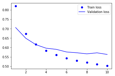
emb_history = deep_model(emb_model, X_train_emb, y_train_emb, X_valid_emb, y_valid_emb)

We have a validation accuracy of about 74%. The number of words in the tweets is rather low, so this result is quite good. By comparing the training and validation loss, we see that the model starts overfitting from epoch 6.
In a previous article, I discussed how we can avoid overfitting. You might want to read that if you want to deep dive on that topic.
When we train the model on all data (including the validation data, but excluding the test data) and set the number of epochs to 6, we get a test accuracy of 78%. This test result is OK, but let’s see if we can improve with pre-trained word embeddings.
emb_results = test_model(emb_model, X_train_seq_trunc, y_train_oh, X_test_seq_trunc, y_test_oh, 6)
print('/n')
print('Test accuracy of word embeddings model: {0:.2f}%'.format(emb_results[1]*100))
Pre-trained word embeddings — Glove
Because the training data is not so large, the model might not be able to learn good embeddings for the sentiment analysis. Alternatively, we can load pre-trained word embeddings built on a much larger training data.
The GloVe database contains multiple pre-trained word embeddings, and more specific embeddings trained on tweets. So this might be useful for the task at hand.
First, we put the word embeddings in a dictionary where the keys are the words and the values the word embeddings.
glove_file = 'glove.twitter.27B.' + str(GLOVE_DIM) + 'd.txt'
emb_dict = {}
glove = open(input_path / glove_file)
for line in glove:
    values = line.split()
    word = values[0]
    vector = np.asarray(values[1:], dtype='float32')
    emb_dict[word] = vector
glove.close()
With the GloVe embeddings loaded in a dictionary, we can look up the embedding for each word in the corpus of the airline tweets. These will be stored in a matrix with a shape of _NBWORDS and _GLOVEDIM. If a word is not found in the GloVe dictionary, the word embedding values for the word are zero.
emb_matrix = np.zeros((NB_WORDS, GLOVE_DIM))
for w, i in tk.word_index.items():
    if i < NB_WORDS:
        vect = emb_dict.get(w)
        if vect is not None:
        emb_matrix[i] = vect
    else:
        break
Then we specify the model just like we did with the model above.
glove_model = models.Sequential()
glove_model.add(layers.Embedding(NB_WORDS, GLOVE_DIM, input_length=MAX_LEN))
glove_model.add(layers.Flatten())
glove_model.add(layers.Dense(3, activation='softmax'))
In the Embedding layer (which is layer 0 here) we set the weights for the words to those found in the GloVe word embeddings. By setting trainable to False we make sure that the GloVe word embeddings cannot be changed. After that, we run the model.
glove_model.layers[0].set_weights([emb_matrix])
glove_model.layers[0].trainable = False
glove_history = deep_model(glove_model, X_train_emb, y_train_emb, X_valid_emb, y_valid_emb)
The model overfits fast after 3 epochs. Furthermore, the validation accuracy is lower compared to the embeddings trained on the training data.
glove_results = test_model(glove_model, X_train_seq_trunc, y_train_oh, X_test_seq_trunc, y_test_oh, 3)
print('/n')
print('Test accuracy of word glove model: {0:.2f}%'.format(glove_results[1]*100))
As a final exercise, let’s see what results we get when we train the embeddings with the same number of dimensions as the GloVe data.
Training word embeddings with more dimensions
We will train the word embeddings with the same number of dimensions as the GloVe embeddings (i.e. GLOVE_DIM).
emb_model2 = models.Sequential()
emb_model2.add(layers.Embedding(NB_WORDS, GLOVE_DIM, input_length=MAX_LEN))
emb_model2.add(layers.Flatten())
emb_model2.add(layers.Dense(3, activation='softmax'))
emb_history2 = deep_model(emb_model2, X_train_emb, y_train_emb, X_valid_emb, y_valid_emb)

emb_results2 = test_model(emb_model2, X_train_seq_trunc, y_train_oh, X_test_seq_trunc, y_test_oh, 3)
print('/n')
print('Test accuracy of word embedding model 2: {0:.2f}%'.format(emb_results2[1]*100))
On the test data we get good results, but we do not outperform the LogisticRegression with the CountVectorizer. So there is still room for improvement.
Conclusion
The best result is achieved with 100-dimensional word embeddings that are trained on the available data. This even outperforms the use of word embeddings that were trained on a much larger Twitter corpus.
Until now we have just put a Dense layer on the flattened embeddings. By doing this, we do not take into account the relationships between the words in the tweet. This can be achieved with a recurrent neural network or a 1D convolutional network. But that’s something for a future post :)