

Karl Pearson was a British mathematician who once said "Statistics is the grammar of science". This holds true especially for Computer and Information Sciences, Physical Science, and Biological Science.
When you are getting started with your journey in Data Science, Data Analytics, Machine Learning, or AI (including Generative AI) having statistical knowledge will help you better leverage data insights and actually understand all the algorithms beyond their implementation approach.
I can't overstate the importance of statistics in data science and Artificial Intelligence. Statistics provides tools and methods to find structure and give deeper data insights. Both Statistics and Mathematics love facts and hate guesses. Knowing the fundamentals of these two important subjects will allow you to think critically, and be creative when using the data to solve business problems and make data-driven decisions.
Key statistical concepts for your data science or data analysis journey with Python Code
In this handbook, I will cover the following Statistics topics for data science, machine learning, and artificial intelligence (including GenAI):
If you have no prior Statistical knowledge and you want to identify and learn the essential statistical concepts from the scratch and prepare for your job interviews, then this handbook is for you. It will also be a good read for anyone who wants to refresh their statistical knowledge.
Prerequisites
Before you start reading this handbook about key concepts in Statistics for Data Science, Machine Learning, and Artificial Intelligence, there are a few prerequisites that will help you make the most out of it.
This list is designed to ensure you are well-prepared and can fully grasp the statistical concepts discussed:
Basic Mathematical Skills: Comfort with high school level mathematics, including algebra and basic calculus, is essential. These skills are crucial for understanding statistical formulas and methods.
Logical Thinking: Ability to think logically and methodically to solve problems will aid in understanding statistical reasoning and applying these concepts to data-driven scenarios.
Computer Literacy: Basic knowledge of using computers and the internet is necessary since many examples and exercises might require the use of statistical software or coding.
Basic knowledge of Python, such as the creation of variables and working with some basic data structures and coding is also required (if you are not familiar with these concepts, check out my Python for Data Science 2024 -Full Course for Beginners here).
Curiosity and Willingness to Learn: A keen interest in learning and exploring data is perhaps the most important prerequisite. The field of data science is constantly evolving, and a proactive approach to learning will be incredibly beneficial.
This handbook assumes no prior knowledge of statistics, making it accessible to beginners. Still, familiarity with the above concepts will greatly enhance your understanding and ability to apply statistical methods effectively in various domains.
If you want to learn Mathematics, Statistics, Machine Learning or AI check out our YouTube Channel and LunarTech.ai for free resources.
Random Variables
Random variables form the cornerstone of many statistical concepts. It might be hard to digest the formal mathematical definition of a random variable, but simply put, it's a way to map the outcomes of random processes, such as flipping a coin or rolling a dice, to numbers.
For instance, we can define the random process of flipping a coin by random variable X which takes a value 1 if the outcome is heads and 0 if the outcome is tails.
$$X = \begin{cases} 1 & \text{if heads} \\ 0 & \text{if tails} \end{cases}$$
In this example, we have a random process of flipping a coin where this experiment can produce two possible outcomes: {0,1}. This set of all possible outcomes is called the sample space of the experiment. Each time the random process is repeated, it is referred to as an event.
In this example, flipping a coin and getting a tail as an outcome is an event. The chance or the likelihood of this event occurring with a particular outcome is called the probability of that event.
A probability of an event is the likelihood that a random variable takes a specific value of x which can be described by P(x). In the example of flipping a coin, the likelihood of getting heads or tails is the same, that is 0.5 or 50%. So we have the following setting:
$$\begin{align} \Pr(X = \text{heads}) = 0.5 \\ \Pr(X = \text{tails}) = 0.5 \end{align}$$
where the probability of an event, in this example, can only take values in the range [0,1].
Mean, Variance, Standard Deviation
To understand the concepts of mean, variance, and many other statistical topics, it is important to learn the concepts of population and sample.
The population is the set of all observations (individuals, objects, events, or procedures) and is usually very large and diverse. On the other hand, a sample is a subset of observations from the population that ideally is a true representation of the population.
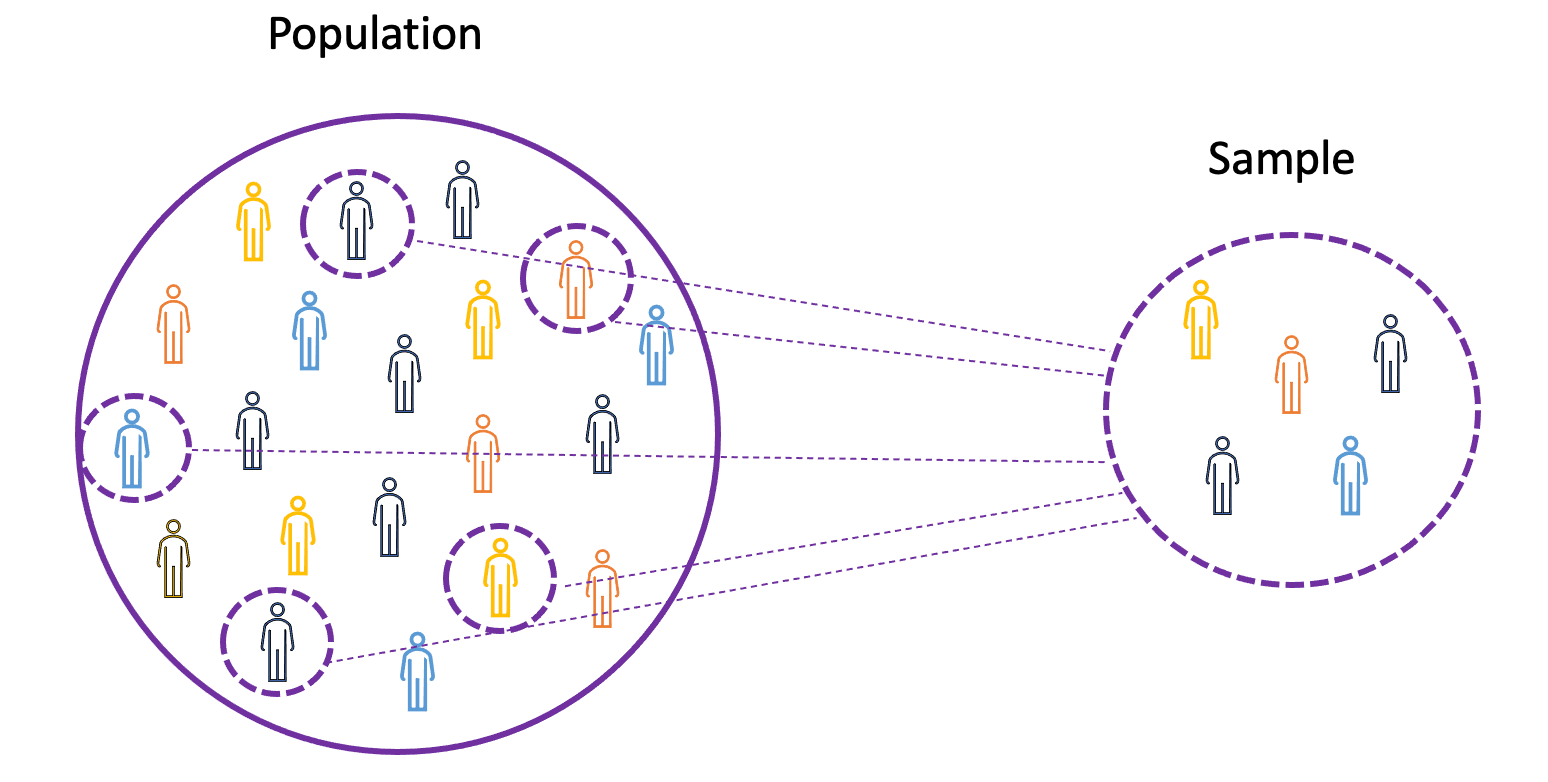
Image Source: LunarTech
Given that experimenting with an entire population is either impossible or simply too expensive, researchers or analysts use samples rather than the entire population in their experiments or trials.
To make sure that the experimental results are reliable and hold for the entire population, the sample needs to be a true representation of the population. That is, the sample needs to be unbiased.
For this purpose, we can use statistical sampling techniques such as Random Sampling, Systematic Sampling, Clustered Sampling, Weighted Sampling, and Stratified Sampling.
Mean
The mean, also known as the average, is a central value of a finite set of numbers. Let’s assume a random variable X in the data has the following values:
$$X_1, X_2, X_3, \ldots, X_N$$
where N is the number of observations or data points in the sample set or simply the data frequency. Then the sample mean defined by μ, which is very often used to approximate the population mean, can be expressed as follows:
$$\mu = \frac{\sum_{i=1}^{N} x_i}{N}$$
The mean is also referred to as expectation which is often defined by E() or random variable with a bar on the top. For example, the expectation of random variables X and Y, that is E(X) and E(Y), respectively, can be expressed as follows:
$$\bar{X} = \frac{\sum_{i=1}^{N} X_i}{N}$$
$$\bar{Y} = \frac{\sum_{i=1}^{N} Y_i}{N}$$
Now that we have a solid understanding of the mean as a statistical measure, let's see how we can apply this knowledge practically using Python. Python is a versatile programming language that, with the help of libraries like NumPy, makes it easy to perform complex mathematical operations—including calculating the mean.
In the following code snippet, we demonstrate how to compute the mean of a set of numbers using NumPy. We will start by showing the calculation for a simple array of numbers. Then, we'll address a common scenario encountered in data science: calculating the mean of a dataset that includes undefined or missing values, represented as NaN (Not a Number). NumPy provides a function specifically designed to handle such cases, allowing us to compute the mean while ignoring these NaN values.
Here is how you can perform these operations in Python:
import numpy as np
import math
x = np.array([1,3,5,6])
mean_x = np.mean(x)

# in case the data contains Nan values
x_nan = np.array([1,3,5,6, math.nan])
mean_x_nan = np.nanmean(x_nan)
Variance
The variance measures how far the data points are spread out from the average value. It's equal to the sum of the squares of the differences between the data values and the average (the mean).
We can express the population variance as follows:
x = np.array([1,3,5,6])
variance_x = np.var(x)

# here you need to specify the degrees of freedom (df) max number of logically independent data points that have freedom to vary
x_nan = np.array([1,3,5,6, math.nan])
mean_x_nan = np.nanvar(x_nan, ddof = 1)
For deriving expectations and variances of different popular probability distribution functions, check out this Github repo.
Standard Deviation
The standard deviation is simply the square root of the variance and measures the extent to which data varies from its mean. The standard deviation defined by sigma can be expressed as follows:
$$\sigma^2 = \frac{\sum_{i=1}^{N} (x_i - \mu)^2}{N}$$
Standard deviation is often preferred over the variance because it has the same units as the data points, which means you can interpret it more easily.
To compute the population variance using Python, we utilize the var function from the NumPy library. By default, this function calculates the population variance by setting the ddof (Delta Degrees of Freedom) parameter to 0. However, when dealing with samples and not the entire population, you would typically set ddof to 1 to get the sample variance.
The code snippet provided shows how to calculate the variance for a set of data. Additionally, it shows how to calculate the variance when there are NaN values in the data. NaN values represent missing or undefined data. When calculating the variance, these NaN values must be handled correctly; otherwise, they can result in a variance that is not a number (NaN), which is uninformative.
Here is how you can calculate the population variance in Python, taking into account the potential presence of NaN values:
x = np.array([1,3,5,6])
variance_x = np.std(x)

x_nan = np.array([1,3,5,6, math.nan])
mean_x_nan = np.nanstd(x_nan, ddof = 1)
Covariance
The covariance is a measure of the joint variability of two random variables and describes the relationship between these two variables. It is defined as the expected value of the product of the two random variables’ deviations from their means.
The covariance between two random variables X and Z can be described by the following expression, where E(X) and E(Z) represent the means of X and Z, respectively.
$$\text{Cov}(X, Z) = E\left[(X - E(X))(Z - E(Z))\right]$$
Covariance can take negative or positive values as well as a value of 0. A positive value of covariance indicates that two random variables tend to vary in the same direction, whereas a negative value suggests that these variables vary in opposite directions. Finally, the value 0 means that they don’t vary together.
To explore the concept of covariance practically, we will use Python with the NumPy library, which provides powerful numerical operations. The np.cov function can be used to calculate the covariance matrix for two or more datasets. In the matrix, the diagonal elements represent the variance of each dataset, and the off-diagonal elements represent the covariance between each pair of datasets.
Let's look at an example of calculating the covariance between two sets of data:
x = np.array([1,3,5,6])
y = np.array([-2,-4,-5,-6])

#this will return the covariance matrix of x,y containing x_variance, y_variance on diagonal elements and covariance of x,y
cov_xy = np.cov(x,y)
Correlation
The correlation is also a measure of a relationship. It measures both the strength and the direction of the linear relationship between two variables.
If a correlation is detected, then it means that there is a relationship or a pattern between the values of two target variables. Correlation between two random variables X and Z is equal to the covariance between these two variables divided by the product of the standard deviations of these variables. This can be described by the following expression:
$$\rho_{X,Z} = \frac{\text{Cov}(X, Z)}{\sigma_X \sigma_Z}$$
Correlation coefficients’ values range between -1 and 1. Keep in mind that the correlation of a variable with itself is always 1, that is Cor(X, X) = 1.
Another thing to keep in mind when interpreting correlation is to not confuse it with causation, given that a correlation is not necessarily a causation. Even if there is a correlation between two variables, you cannot conclude that one variable causes a change in the other. This relationship could be coincidental, or a third factor might be causing both variables to change.
x = np.array([1,3,5,6])
y = np.array([-2,-4,-5,-6])

corr = np.corrcoef(x,y)
Probability Distribution Functions
A function that describes all the possible values, the sample space, and the corresponding probabilities that a random variable can take within a given range, bounded between the minimum and maximum possible values, is called a probability distribution function (pdf) or probability density.
Every pdf needs to satisfy the following two criteria:
$$0 \leq \Pr(X) \leq 1 \\ \sum p(X) = 1$$
where the first criterium states that all probabilities should be numbers in the range of [0,1] and the second criterium states that the sum of all possible probabilities should be equal to 1.
Probability functions are usually classified into two categories: discrete and continuous.
Discrete distribution function describes the random process with countable sample space, like in an example of tossing a coin that has only two possible outcomes. Continuous distribution functions describe the random process with a continuous sample space.
Examples of discrete distribution functions are Bernoulli, Binomial, Poisson, Discrete Uniform. Examples of continuous distribution functions are Normal, Continuous Uniform, Cauchy.
Binomial Distribution
The binomial distribution is the discrete probability distribution of the number of successes in a sequence of n independent experiments, each with the boolean-valued outcome: success (with probability p) or failure (with probability q = 1 − p).
Let's assume a random variable X follows a Binomial distribution, then the probability of observing k successes in n independent trials can be expressed by the following probability density function:
$$\Pr(X = k) = \binom{n}{k} p^k q^{n-k}$$
The binomial distribution is useful when analyzing the results of repeated independent experiments, especially if you're interested in the probability of meeting a particular threshold given a specific error rate.
Binomial Distribution Mean and Variance
The mean of a binomial distribution, denoted as E(X)=np, tells you the average number of successes you can expect if you conduct n independent trials of a binary experiment.
A binary experiment is one where there are only two outcomes: success (with probability p) or failure (with probability q\=1−_p_).
$$E(X) = np \\ \text{Var}(X) = npq$$
For example, if you were to flip a coin 100 times and you define a success as the coin landing on heads (let's say the probability of heads is 0.5), the binomial distribution would tell you how likely it is to get any number of heads in those 100 flips. The mean E(X) would be 100×0.5=50, indicating that on average, you’d expect to get 50 heads.
The variance Var(X)=npq measures the spread of the distribution, indicating how much the number of successes is likely to deviate from the mean.
Continuing with the coin flip example, the variance would be 100×0.5×0.5=25, which informs you about the variability of the outcomes. A smaller variance would mean the results are more tightly clustered around the mean, whereas a larger variance indicates they’re more spread out.
These concepts are crucial in many fields. For instance:
Quality Control: Manufacturers might use the binomial distribution to predict the number of defective items in a batch, helping them understand the quality and consistency of their production process.
Healthcare: In medicine, it could be used to calculate the probability of a certain number of patients responding to a treatment, based on past success rates.
Finance: In finance, binomial models are used to evaluate the risk of portfolio or investment strategies by predicting the number of times an asset will reach a certain price point.
Polling and Survey Analysis: When predicting election results or customer preferences, pollsters might use the binomial distribution to estimate how many people will favor a candidate or a product, given the probability drawn from a sample.
Understanding the mean and variance of the binomial distribution is fundamental to interpreting the results and making informed decisions based on the likelihood of different outcomes.
The figure below visualizes an example of Binomial distribution where the number of independent trials is equal to 8 and the probability of success in each trial is equal to 16%.
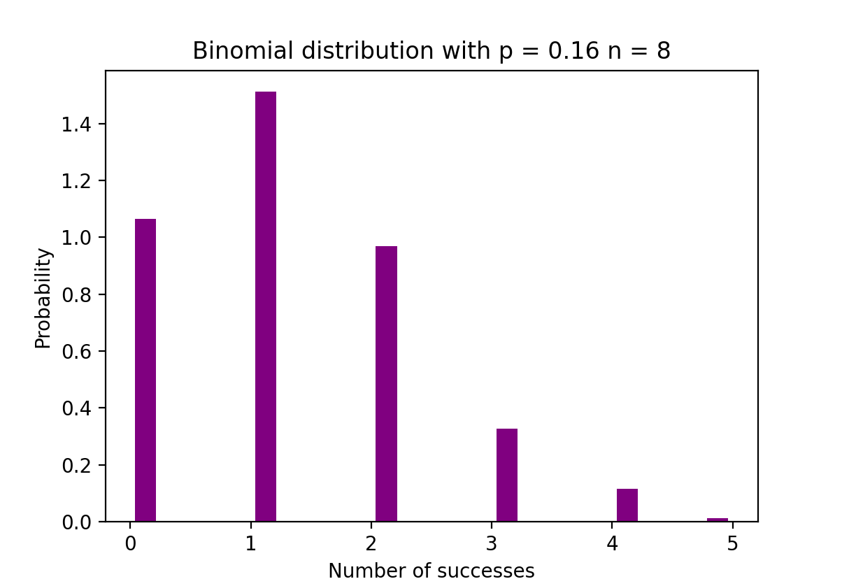
Binomial distribution - showing number of success and probability. Image Source: LunarTech
The Python code below creates a histogram to visualize the distribution of outcomes from 1000 experiments, each consisting of 8 trials with a success probability of 0.16. It uses NumPy to generate the binomial distribution data and Matplotlib to plot the histogram, showing the probability of the number of successes in those trials.
# Random Generation of 1000 independent Binomial samples
import numpy as np
import matplotlib.pyplot as plt


n = 8
p = 0.16
N = 1000
X = np.random.binomial(n,p,N)
# Histogram of Binomial distribution

counts, bins, ignored = plt.hist(X, 20, density = True, rwidth = 0.7, color = 'purple')
plt.title("Binomial distribution with p = 0.16 n = 8")
plt.xlabel("Number of successes")
plt.ylabel("Probability")plt.show()
Poisson Distribution
The Poisson distribution is the discrete probability distribution of the number of events occurring in a specified time period, given the average number of times the event occurs over that time period.
Let's assume a random variable X follows a Poisson distribution. Then the probability of observing k events over a time period can be expressed by the following probability function:
$$\Pr(X = k) = \frac{\lambda^k e^{-\lambda}}{k!}$$
where e is Euler’s number and λ lambda, the arrival rate parameter, is the expected value of X. The Poisson distribution function is very popular for its usage in modeling countable events occurring within a given time interval.
Poisson Distribution Mean and Variance
The Poisson distribution is particularly useful for modeling the number of times an event occurs within a specified time frame. The mean E(X) and variance Var(X)
Var(X) of a Poisson distribution are both equal to λ, which is the average rate at which events occur (also known as the rate parameter). This makes the Poisson distribution unique, as it is characterized by this single parameter.
The fact that the mean and variance are equal means that as we observe more events, the distribution of the number of occurrences becomes more predictable. It’s used in various fields such as business, engineering, and science for tasks like:
Predicting the number of customer arrivals at a store within an hour. Estimating the number of emails you'd receive in a day. Understanding the number of defects in a batch of materials.
So, the Poisson distribution helps in making probabilistic forecasts about the occurrence of rare or random events over intervals of time or space.
$$E(X) = \lambda \\ \text{Var}(X) = \lambda$$
For example, Poisson distribution can be used to model the number of customers arriving in the shop between 7 and 10 pm, or the number of patients arriving in an emergency room between 11 and 12 pm.
The figure below visualizes an example of Poisson distribution where we count the number of Web visitors arriving at the website where the arrival rate, lambda, is assumed to be equal to 7 minutes.

Randomly generating from Poisson Distribution with lambda = 7. Image Source: LunarTech
In practical data analysis, it is often helpful to simulate the distribution of events. Below is a Python code snippet that demonstrates how to generate a series of data points that follow a Poisson distribution using NumPy. We then create a histogram using Matplotlib to visualize the distribution of the number of visitors (as an example) we might expect to see, based on our average rate λ = 7
This histogram helps in understanding the distribution's shape and variability. The most likely number of visitors is around the mean λ, but the distribution shows the probability of seeing fewer or greater numbers as well.
# Random Generation of 1000 independent Poisson samples
import numpy as np
lambda_ = 7
N = 1000
X = np.random.poisson(lambda_,N)

# Histogram of Poisson distribution
import matplotlib.pyplot as plt
counts, bins, ignored = plt.hist(X, 50, density = True, color = 'purple')
plt.title("Randomly generating from Poisson Distribution with lambda = 7")
plt.xlabel("Number of visitors")
plt.ylabel("Probability")
plt.show()
Normal Distribution
The Normal probability distribution is the continuous probability distribution for a real-valued random variable. Normal distribution, also called Gaussian distribution is arguably one of the most popular distribution functions that is commonly used in social and natural sciences for modeling purposes. For example, it is used to model people’s height or test scores.
Let's assume a random variable X follows a Normal distribution. Then its probability density function can be expressed as follows:
$$\Pr(X = k) = \frac{1}{\sigma\sqrt{2\pi}} e^{-\frac{1}{2} \left(\frac{x-\mu}{\sigma}\right)^2}$$
where the parameter μ (mu) is the mean of the distribution also referred to as the location parameter, parameter σ (sigma) is the standard deviation of the distribution also referred to as the scale parameter. The number π (pi) is a mathematical constant approximately equal to 3.14.
Normal Distribution Mean and Variance
$$E(X) = \mu \\ \text{Var}(X) = \sigma^2$$
The figure below visualizes an example of Normal distribution with a mean 0 (μ = 0) and standard deviation of 1 (σ = 1), which is referred to as Standard Normal distribution which is symmetric_._
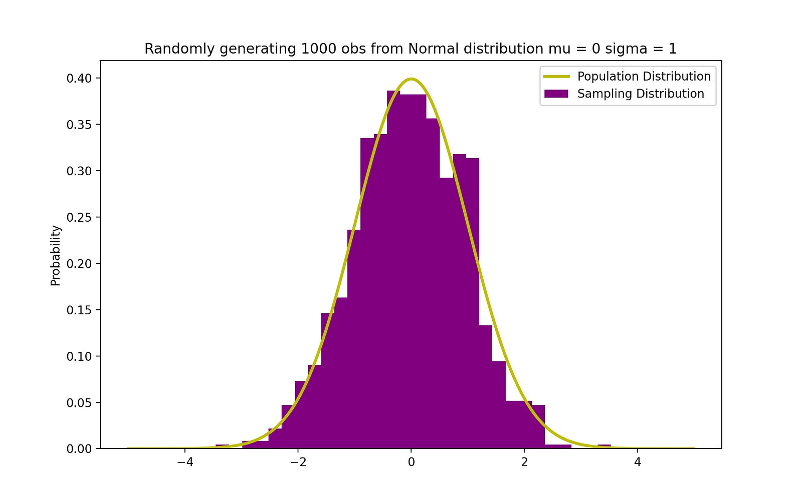
Randomly generating 1000 obs from Normal Distribution (mu = 0, sigma = 1). Image Source: LunarTech
The visualization of the standard normal distribution is crucial because this distribution underpins many statistical methods and probability theory. When data is normally distributed with a mean ( μ ) of 0 and standard deviation (σ) of 1, it is referred to as the standard normal distribution. It's symmetric around the mean, with the shape of the curve often called the "bell curve" due to its bell-like shape.
The standard normal distribution is fundamental for the following reasons:
Central Limit Theorem: This theorem states that, under certain conditions, the sum of a large number of random variables will be approximately normally distributed. It allows for the use of normal probability theory for sample means and sums, even when the original data is not normally distributed.
Z-Scores: Values from any normal distribution can be transformed into the standard normal distribution using Z-scores, which indicate how many standard deviations an element is from the mean. This allows for the comparison of scores from different normal distributions.
Statistical Inference and AB Testing: Many statistical tests, such as t-tests and ANOVAs, assume that the data follows a normal distribution, or they rely on the central limit theorem. Understanding the standard normal distribution helps in the interpretation of these tests' results.
Confidence Intervals and Hypothesis Testing: The properties of the standard normal distribution are used to construct confidence intervals and to perform hypothesis testing.
All topics which we will cover below!
So, being able to visualize and understand the standard normal distribution is key to applying many statistical techniques accurately.
The Python code below uses NumPy to generate 1000 random samples from a normal distribution with a mean (μ) of 0 and a standard deviation (σ) of 1, which are standard parameters for the standard normal distribution. These generated samples are stored in the variable X.
To visualize the distribution of these samples, the code employs Matplotlib to create a histogram. The plt.hist function is used to plot the histogram of the samples with 30 bins, and the density parameter is set to True to normalize the histogram so that the area under it sums to 1. This effectively turns the histogram into a probability density plot.
Additionally, the SciPy library is used to overlay the probability density function (PDF) of the theoretical normal distribution on the histogram. The norm.pdf function generates the y-values for the PDF given an array of x-values. This theoretical curve is plotted in yellow over the histogram to show how closely the random samples fit the expected distribution.
The resulting graph displays the histogram of the generated samples in purple, with the theoretical normal distribution overlaid in yellow. The x-axis represents the range of values that the samples can take, while the y-axis represents the probability density. This visualization is a powerful tool for comparing the empirical distribution of the data with the theoretical model, allowing us to see whether our samples follow the expected pattern of a normal distribution.
# Random Generation of 1000 independent Normal samples
import numpy as np
mu = 0
sigma = 1
N = 1000
X = np.random.normal(mu,sigma,N)

# Population distribution
from scipy.stats import norm
x_values = np.arange(-5,5,0.01)
y_values = norm.pdf(x_values)
#Sample histogram with Population distribution
import matplotlib.pyplot as plt
counts, bins, ignored = plt.hist(X, 30, density = True,color = 'purple',label = 'Sampling Distribution')
plt.plot(x_values,y_values, color = 'y',linewidth = 2.5,label = 'Population Distribution')
plt.title("Randomly generating 1000 obs from Normal distribution mu = 0 sigma = 1")
plt.ylabel("Probability")
plt.legend()
plt.show()
Bayes' Theorem
The Bayes' Theorem (often called Bayes' Law) is arguably the most powerful rule of probability and statistics. It was named after famous English statistician and philosopher, Thomas Bayes.

English mathematician and philosopher Thomas Bayes
Bayes' theorem is a powerful probability law that brings the concept of subjectivity into the world of Statistics and Mathematics where everything is about facts. It describes the probability of an event, based on the prior information of conditions that might be related to that event.
For instance, if the risk of getting Coronavirus or Covid-19 is known to increase with age, then Bayes' Theorem allows the risk to an individual of a known age to be determined more accurately. It does this by conditioning it on the age rather than simply assuming that this individual is common to the population as a whole.
The concept of conditional probability, which plays a central role in Bayes' theorem, is a measure of the probability of an event happening, given that another event has already occurred.
Bayes' theorem can be described by the following expression where the X and Y stand for events X and Y, respectively:
$$\Pr(X | Y) = \frac{\Pr(Y | X) \Pr(X)}{\Pr(Y)}$$
Pr (X|Y): the probability of event X occurring given that event or condition Y has occurred or is true
Pr (Y|X): the probability of event Y occurring given that event or condition X has occurred or is true
Pr (X) & Pr (Y): the probabilities of observing events X and Y, respectively
In the case of the earlier example, the probability of getting Coronavirus (event X) conditional on being at a certain age is Pr (X|Y). This is equal to the probability of being at a certain age given that the person got a Coronavirus, Pr (Y|X), multiplied with the probability of getting a Coronavirus, Pr (X), divided by the probability of being at a certain age, Pr (Y).
Linear Regression
Earlier, we introduced the concept of causation between variables, which happens when a variable has a direct impact on another variable.
When the relationship between two variables is linear, then Linear Regression is a statistical method that can help model the impact of a unit change in a variable, the independent variable on the values of another variable, the dependent variable.
Dependent variables are often referred to as response variables or explained variables, whereas independent variables are often referred to as regressors or explanatory variables.
When the Linear Regression model is based on a single independent variable, then the model is called Simple Linear Regression. When the model is based on multiple independent variables, it’s referred to as Multiple Linear Regression.
Simple Linear Regression can be described by the following expression:
$$Y_i = \beta_0 + \beta_1X_i + u_i$$
where Y is the dependent variable, X is the independent variable which is part of the data, β0 is the intercept which is unknown and constant, β1 is the slope coefficient or a parameter corresponding to the variable X which is unknown and constant as well. Finally, u is the error term that the model makes when estimating the Y values.
The main idea behind linear regression is to find the best-fitting straight line, the regression line, through a set of paired ( X, Y ) data.
One example of the Linear Regression application is modeling the impact of flipper length on penguins’ body mass, which is visualized below:
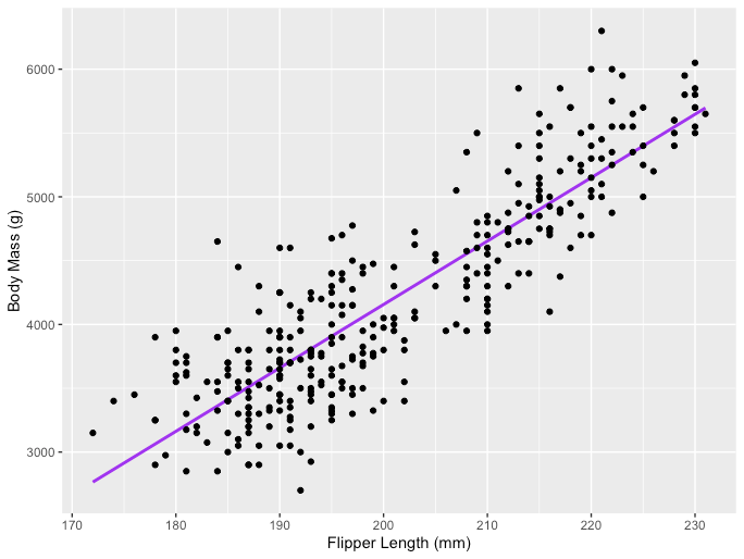
Image Source: LunarTech
The R code snippet you've shared is for creating a scatter plot with a linear regression line using the ggplot2 package in R, which is a powerful and widely-used library for creating graphics and visualizations. The code uses a dataset named penguins from the palmerpenguins package, presumably containing data about penguin species, including measurements like flipper length and body mass.
# R code for the graph
install.packages("ggplot2")
install.packages("palmerpenguins")
library(palmerpenguins)
library(ggplot2)
View(data(penguins))
ggplot(data = penguins, aes(x = flipper_length_mm,y = body_mass_g))+
  geom_smooth(method = "lm", se = FALSE, color = 'purple')+
  geom_point()+
  labs(x="Flipper Length (mm)",y="Body Mass (g)")
Multiple Linear Regression with three independent variables can be described by the following expression:
$$Y_i = \beta_0 + \beta_1X_{1,i} + \beta_2X_{2,i} + \beta_3X_{3,i} + u_i$$
Ordinary Least Squares
The ordinary least squares (OLS) is a method for estimating the unknown parameters such as β0 and β1 in a linear regression model. The model is based on the principle of least squares. This minimizes the sum of the squares of the differences between the observed dependent variable and its values that are predicted by the linear function of the independent variable (often referred to as fitted values).
This difference between the real and predicted values of dependent variable Y is referred to as residual. So OLS minimizes the sum of squared residuals.
This optimization problem results in the following OLS estimates for the unknown parameters β0 and β1 which are also known as coefficient estimates:
$$\hat{\beta}1 = \frac{\sum{i=1}^{N} (X_i - \bar{X})(Y_i - \bar{Y})}{\sum_{i=1}^{N} (X_i - \bar{X})^2}$$
$$\hat{\beta}_0 = \bar{Y} - \hat{\beta}_1\bar{X}$$
Once these parameters of the Simple Linear Regression model are estimated, the fitted values of the response variable can be computed as follows:
$$\hat{Y}_i = \hat{\beta}_0 + \hat{\beta}_1X_i$$
Standard Error
The residuals or the estimated error terms can be determined as follows:
$$\hat{u}_i = Y_i - \hat{Y}_i$$
It is important to keep in mind the difference between the error terms and residuals. Error terms are never observed, while the residuals are calculated from the data. The OLS estimates the error terms for each observation but not the actual error term. So, the true error variance is still unknown.
Also, these estimates are subject to sampling uncertainty. This means that we will never be able to determine the exact estimate, the true value, of these parameters from sample data in an empirical application. But we can estimate it by calculating the sample residual variance by using the residuals as follows:
$$\hat{\sigma}^2 = \frac{\sum_{i=1}^{N} \hat{u}_i^2}{N - 2}$$
This estimate for the variance of sample residuals helps us estimate the variance of the estimated parameters, which is often expressed as follows:
$$\text{Var}(\hat{\beta})$$
The square root of this variance term is called the standard error of the estimate. This is a key component in assessing the accuracy of the parameter estimates. It is used to calculate test statistics and confidence intervals.
The standard error can be expressed as follows:
$$SE(\hat{\beta}) = \sqrt{\text{Var}(\hat{\beta})}$$
It is important to keep in mind the difference between the error terms and residuals. Error terms are never observed, while the residuals are calculated from the data.
OLS Assumptions
The OLS estimation method makes the following assumptions which need to be satisfied to get reliable prediction results:
The Linearity assumption states that the model is linear in parameters.
The Random Sample assumption states that all observations in the sample are randomly selected.
The Exogeneity assumption states that independent variables are uncorrelated with the error terms.
The Homoskedasticity assumption states that the variance of all error terms is constant.
The No Perfect Multi-Collinearity assumption states that none of the independent variables is constant and there are no exact linear relationships between the independent variables.
The Python code snippet you've shared performs Ordinary Least Squares (OLS) regression, which is a method used in statistics to estimate the relationship between independent variables and a dependent variable. This process involves calculating the best-fit line through the data points that minimizes the sum of the squared differences between the observed values and the values predicted by the model.
The code defines a function runOLS(Y, X) that takes in a dependent variable Y and an independent variable X and performs the following steps:
Estimates the OLS coefficients (beta_hat) using the linear algebra solution to the least squares problem.
Makes predictions (
Y_hat) using the estimated coefficients and calculates the residuals.Computes the residual sum of squares (RSS), total sum of squares (TSS), mean squared error (MSE), root mean squared error (RMSE), and R-squared value, which are common metrics used to assess the fit of the model.
Calculates the standard error of the coefficient estimates, t-statistics, p-values, and confidence intervals for the estimated coefficients.
These calculations are standard in regression analysis and are used to interpret and understand the strength and significance of the relationship between the variables. The result of this function includes the estimated coefficients and various statistics that help evaluate the model's performance.
def runOLS(Y,X):

   # OLS esyimation Y = Xb + e --> beta_hat = (X'X)^-1(X'Y)
   beta_hat = np.dot(np.linalg.inv(np.dot(np.transpose(X), X)), np.dot(np.transpose(X), Y))

   # OLS prediction
   Y_hat = np.dot(X,beta_hat)
   residuals = Y-Y_hat
   RSS = np.sum(np.square(residuals))
   sigma_squared_hat = RSS/(N-2)
   TSS = np.sum(np.square(Y-np.repeat(Y.mean(),len(Y))))
   MSE = sigma_squared_hat
   RMSE = np.sqrt(MSE)
   R_squared = (TSS-RSS)/TSS

   # Standard error of estimates:square root of estimate's variance
   var_beta_hat = np.linalg.inv(np.dot(np.transpose(X),X))*sigma_squared_hat

   SE = []
   t_stats = []
   p_values = []
   CI_s = []

   for i in range(len(beta)):
       #standard errors
       SE_i = np.sqrt(var_beta_hat[i,i])
       SE.append(np.round(SE_i,3))

        #t-statistics
        t_stat = np.round(beta_hat[i,0]/SE_i,3)
        t_stats.append(t_stat)

        #p-value of t-stat p[|t_stat| >= t-treshhold two sided]
        p_value = t.sf(np.abs(t_stat),N-2) * 2
        p_values.append(np.round(p_value,3))

        #Confidence intervals = beta_hat -+ margin_of_error
        t_critical = t.ppf(q =1-0.05/2, df = N-2)
        margin_of_error = t_critical*SE_i
        CI = [np.round(beta_hat[i,0]-margin_of_error,3), np.round(beta_hat[i,0]+margin_of_error,3)]
        CI_s.append(CI)
        return(beta_hat, SE, t_stats, p_values,CI_s,
               MSE, RMSE, R_squared)
Parameter Properties
Under the assumption that the OLS criteria/assumptions we just discussed are satisfied, the OLS estimators of coefficients β0 and β1 are BLUE and Consistent. So what does this mean?
Gauss-Markov Theorem
This theorem highlights the properties of OLS estimates where the term BLUE stands for Best Linear Unbiased Estimator. Let's explore what this means in more detail.
Bias
The bias of an estimator is the difference between its expected value and the true value of the parameter being estimated. It can be expressed as follows:
$$\text{Bias}(\beta, \hat{\beta}) = E(\hat{\beta}) - \beta$$
When we state that the estimator is unbiased, we mean that the bias is equal to zero. This implies that the expected value of the estimator is equal to the true parameter value, that is:
$$E(\hat{\beta}) = \beta$$
Unbiasedness does not guarantee that the obtained estimate with any particular sample is equal or close to β. What it means is that, if we repeatedly draw random samples from the population and then computes the estimate each time, then the average of these estimates would be equal or very close to β.
Efficiency
The term Best in the Gauss-Markov theorem relates to the variance of the estimator and is referred to as efficiency*.* A parameter can have multiple estimators but the one with the lowest variance is called efficient.
Consistency
The term consistency goes hand in hand with the terms sample size and convergence. If the estimator converges to the true parameter as the sample size becomes very large, then this estimator is said to be consistent, that is:
$$N \to \infty \text{ then } \hat{\beta} \to \beta$$
All these properties hold for OLS estimates as summarized in the Gauss-Markov theorem. In other words, OLS estimates have the smallest variance, they are unbiased, linear in parameters, and are consistent. These properties can be mathematically proven by using the OLS assumptions made earlier.
Confidence Intervals
The Confidence Interval is the range that contains the true population parameter with a certain pre-specified probability. This is referred to as the confidence level of the experiment, and it's obtained by using the sample results and the margin of error.
Margin of Error
The margin of error is the difference between the sample results and based on what the result would have been if you had used the entire population.
Confidence Level
The Confidence Level describes the level of certainty in the experimental results. For example, a 95% confidence level means that if you were to perform the same experiment repeatedly 100 times, then 95 of those 100 trials would lead to similar results.
Note that the confidence level is defined before the start of the experiment because it will affect how big the margin of error will be at the end of the experiment.
Confidence Interval for OLS Estimates
As I mentioned earlier, the OLS estimates of the Simple Linear Regression, the estimates for intercept β0 and slope coefficient β1, are subject to sampling uncertainty. But we can construct Confidence Intervals (CIs) for these parameters which will contain the true value of these parameters in 95% of all samples.
That is, 95% confidence interval for β can be interpreted as follows:
The confidence interval is the set of values for which a hypothesis test cannot be rejected to the level of 5%.
The confidence interval has a 95% chance to contain the true value of β.
95% confidence interval of OLS estimates can be constructed as follows:
$$CI_{0.95}^{\beta} = \left[\hat{\beta}_i - 1.96 , SE(\hat{\beta}_i), \hat{\beta}_i + 1.96 , SE(\hat{\beta}_i)\right]$$
This is based on the parameter estimate, the standard error of that estimate, and the value 1.96 representing the margin of error corresponding to the 5% rejection rule.
This value is determined using the Normal Distribution table, which we'll discuss later on in this handbook.
Meanwhile, the following figure illustrates the idea of 95% CI:
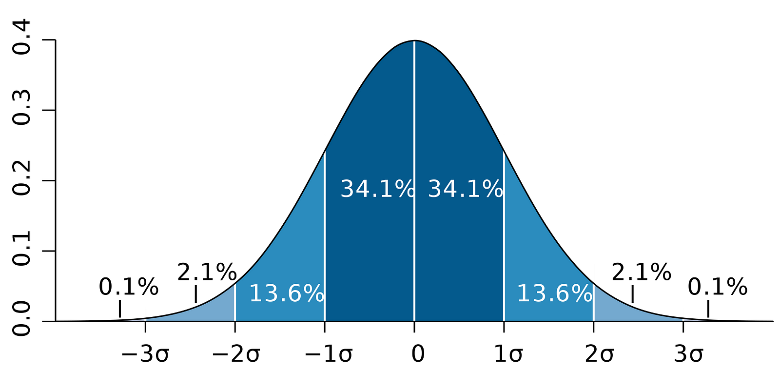
Image Source: LunarTech
Note that the confidence interval depends on the sample size as well, given that it is calculated using the standard error which is based on sample size.
Statistical Hypothesis Testing
Testing a hypothesis in Statistics is a way to test the results of an experiment or survey to determine how meaningful they the results are.
Basically, you're testing whether the obtained results are valid by figuring out the odds that the results have occurred by chance. If it is the letter, then the results are not reliable and neither is the experiment. Hypothesis Testing is part of the Statistical Inference.
Null and Alternative Hypothesis
Firstly, you need to determine the thesis you wish to test. Then you need to formulate the Null Hypothesis and the Alternative Hypothesis. The test can have two possible outcomes. Based on the statistical results, you can either reject the stated hypothesis or accept it.
As a rule of thumb, statisticians tend to put the version or formulation of the hypothesis under the Null Hypothesis that needs to be rejected_,_ whereas the acceptable and desired version is stated under the Alternative Hypothesis_._
Statistical Significance
Let’s look at the earlier mentioned example where we used the Linear Regression model to investigate whether a penguin's Flipper Length, the independent variable, has an impact on Body Mass_,_ the dependent variable.
We can formulate this model with the following statistical expression:
$$Y_{\text{BodyMass}} = \beta_0 + \beta_1X_{\text{FlipperLength}} + u_i$$
Then, once the OLS estimates of the coefficients are estimated, we can formulate the following Null and Alternative Hypothesis to test whether the Flipper Length has a statistically significant impact on the Body Mass:

where H0 and H1 represent Null Hypothesis and Alternative Hypothesis, respectively.
Rejecting the Null Hypothesis would mean that a one-unit increase in Flipper Length has a direct impact on the Body Mass (given that the parameter estimate of β1 is describing this impact of the independent variable, Flipper Length, on the dependent variable, Body Mass). We can reformulate this hypothesis as follows:
$$\begin{cases} H_0: \hat{\beta}_1 = 0 \\ H_1: \hat{\beta}_1 \neq 0 \end{cases}$$
where H0 states that the parameter estimate of β1 is equal to 0, that is Flipper Length effect on Body Mass is statistically insignificant whereas H1 states that the parameter estimate of β1 is not equal to 0, suggesting that Flipper Length effect on Body Mass is statistically significant.
Type I and Type II Errors
When performing Statistical Hypothesis Testing, you need to consider two conceptual types of errors: Type I error and Type II error.
Type I errors occur when the Null is incorrectly rejected, and Type II errors occur when the Null Hypothesis is incorrectly not rejected. A confusion matrix can help you clearly visualize the severity of these two types of errors.
As a rule of thumb, statisticians tend to put the version of the hypothesis under the Null Hypothesis that that needs to be rejected, whereas the acceptable and desired version is stated under the Alternative Hypothesis.
Statistical Tests
Once the you've stataed the Null and the Alternative Hypotheses and defined the test assumptions, the next step is to determine which statistical test is appropriate and to calculate the test statistic.
Whether or not to reject or not reject the Null can be determined by comparing the test statistic with the critical value. This comparison shows whether or not the observed test statistic is more extreme than the defined critical value.
It can have two possible results:
The test statistic is more extreme than the critical value → the null hypothesis can be rejected
The test statistic is not as extreme as the critical value → the null hypothesis cannot be rejected
The critical value is based on a pre-specified significance level α (usually chosen to be equal to 5%) and the type of probability distribution the test statistic follows.
The critical value divides the area under this probability distribution curve into the rejection region(s) and non-rejection region. There are numerous statistical tests used to test various hypotheses. Examples of Statistical tests are Student’s t-test, F-test, Chi-squared test, Durbin-Hausman-Wu Endogeneity test, White Heteroskedasticity test. In this handbook, we will look at two of these statistical tests: the Student's t-test and the F-test.
Student’s t-test
One of the simplest and most popular statistical tests is the Student’s t-test. You can use it to test various hypotheses, especially when dealing with a hypothesis where the main area of interest is to find evidence for the statistically significant effect of a single variable.
The test statistics of the t-test follows Student’s t distribution and can be determined as follows:
$$T_{\text{stat}} = \frac{\hat{\beta}_i - h_0}{SE(\hat{\beta})}$$
where h0 in the nominator is the value against which the parameter estimate is being tested. So, the t-test statistics are equal to the parameter estimate minus the hypothesized value divided by the standard error of the coefficient estimate.
Let's use this for our earlier hypothesis, where we wanted to test whether Flipper Length has a statistically significant impact on Body Mass or not. This test can be performed using a t-test. The h0 is in that case equal to the 0 since the slope coefficient estimate is tested against a value of 0.
Two-sided vs one-sided t-test
There are two versions of the t-test: a two-sided t-test and a one-sided t-test. Whether you need the former or the latter version of the test depends entirely on the hypothesis that you want to test.
You can use the two-sided or two-tailed t-test when the hypothesis is testing equal versus not equal relationship under the Null and Alternative Hypotheses. It would be similar to the following example:
$$H_{0} = \beta_hat_1 = h_0\ H_{1} = \beta_hat_1 \neq h_0$$
The two-sided t-test has two rejection regions as visualized in the figure below:
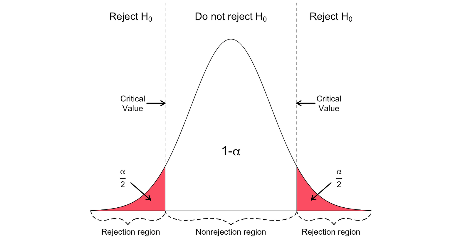
_Image Source: [Hartmann, K., Krois, J., Waske, B. (2018): E-Learning Project SOGA: Statistics and Geospatial Data Analysis. Department of Earth Sciences, Freie Universitaet Berlin](https://www.geo.fu-berlin.de/en/v/soga/Basics-of-statistics/Hypothesis-Tests/Introduction-to-Hypothesis-Testing/Critical-Value-and-the-p-Value-Approach/index.html" data-href="https://www.geo.fu-berlin.de/en/v/soga/Basics-of-statistics/Hypothesis-Tests/Introduction-to-Hypothesis-Testing/Critical-Value-and-the-p-Value-Approach/index.html" class="markup--anchor markup--figure-anchor" rel="noopener" target="blank"><em class="markup--em markup--figure-em)
In this version of the t-test, the Null is rejected if the calculated t-statistics is either too small or too large.
$$T_{\text{stat}} < -t_{\alpha,N} \text{ or } T_{\text{stat}} > t_{\alpha,N}$$
$$|T_{\text{stat}}| > t_{\alpha,N}$$
Here, the test statistics are compared to the critical values based on the sample size and the chosen significance level. To determine the exact value of the cutoff point, you can use a two-sided t-distribution table.
On the other hand, you can use the one-sided or one-tailed t-test when the hypothesis is testing positive/negative versus negative/positive relationships under the Null and Alternative Hypotheses. It looks like this:

Left-tailed vs right-tailed
One-sided t-test has a single rejection region. Depending on the hypothesis side, the rejection region is either on the left-hand side or the right-hand side as visualized in the figure below:
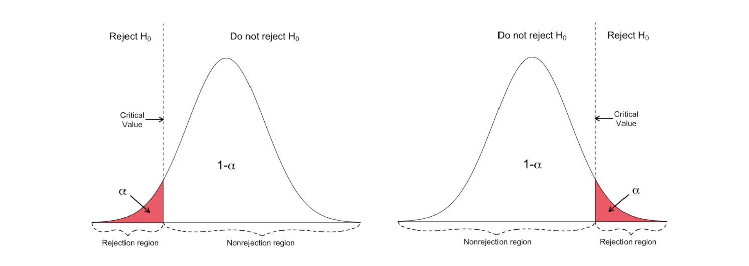
_Image Source: [Hartmann, K., Krois, J., Waske, B. (2018): E-Learning Project SOGA: Statistics and Geospatial Data Analysis. Department of Earth Sciences, Freie Universitaet Berlin](https://www.geo.fu-berlin.de/en/v/soga/Basics-of-statistics/Hypothesis-Tests/Introduction-to-Hypothesis-Testing/Critical-Value-and-the-p-Value-Approach/index.html" data-href="https://www.geo.fu-berlin.de/en/v/soga/Basics-of-statistics/Hypothesis-Tests/Introduction-to-Hypothesis-Testing/Critical-Value-and-the-p-Value-Approach/index.html" class="markup--anchor markup--figure-anchor" rel="noopener" target="blank"><em class="markup--em markup--figure-em)
In this version of the t-test, the Null is rejected if the calculated t-statistics is smaller/larger than the critical value.

F-test
F-test is another very popular statistical test often used to test hypotheses testing a joint statistical significance of multiple variables. This is the case when you want to test whether multiple independent variables have a statistically significant impact on a dependent variable.
Following is an example of a statistical hypothesis that you can test using the F-test:
$$\begin{cases} H_0: \hat{\beta}_1 = \hat{\beta}_2 = \hat{\beta}_3 = 0 \\ H_1: \hat{\beta}_1 \neq \hat{\beta}_2 \neq \hat{\beta}_3 \neq 0 \end{cases}$$
where the Null states that the three variables corresponding to these coefficients are jointly statistically insignificant, and the Alternative states that these three variables are jointly statistically significant.
The test statistics of the F-test follows F distribution and can be determined as follows:
$$F_{\text{stat}} = \frac{(SSR_{\text{restricted}} - SSR_{\text{unrestricted}}) / q}{SSR_{\text{unrestricted}} / (N - k_{\text{unrestricted}} - 1)}$$
where :
the SSRrestricted is the sum of squared residuals of the restricted model, which is the same model excluding from the data the target variables stated as insignificant under the Null
the SSRunrestricted is the sum of squared residuals of the unrestricted model, which is the model that includes all variables
the q represents the number of variables that are being jointly tested for the insignificance under the Null
N is the sample size
and the k is the total number of variables in the unrestricted model.
SSR values are provided next to the parameter estimates after running the OLS regression, and the same holds for the F-statistics as well.
Following is an example of MLR model output where the SSR and F-statistics values are marked.
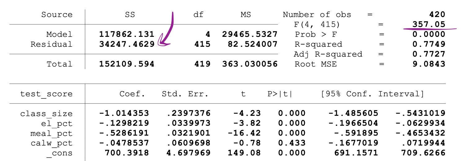
_Image Source:[ Stock and Whatson](https://www.uio.no/studier/emner/sv/oekonomi/ECON4150/v18/lecture7_ols_multiple_regressors_hypothesis_tests.pdf" data-href="https://www.uio.no/studier/emner/sv/oekonomi/ECON4150/v18/lecture7_ols_multiple_regressors_hypothesis_tests.pdf" class="markup--anchor markup--figure-anchor" rel="noopener" target="blank)
F-test has a single rejection region as visualized below:
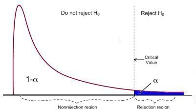
_Image Source: [U of Michigan](https://www.statisticshowto.com/probability-and-statistics/f-statistic-value-test/" data-href="https://www.statisticshowto.com/probability-and-statistics/f-statistic-value-test/" class="markup--anchor markup--figure-anchor" rel="noopener" target="blank"><em class="markup--em markup--figure-em)
If the calculated F-statistics is bigger than the critical value, then the Null can be rejected. This suggests that the independent variables are jointly statistically significant. The rejection rule can be expressed as follows:
$$F_{\text{stat}} > F_{\alpha,q,N}$$
2-sample T-test
If you want to test whether there is a statistically significant difference between the control and experimental groups’ metrics that are in the form of averages (for example, average purchase amount), metric follows student-t distribution. When the sample size is smaller than 30, you can use 2-sample T-test to test the following hypothesis:
$$\begin{cases} H_0: \mu_{\text{con}} = \mu_{\text{exp}} \\ H_1: \mu_{\text{con}} \neq \mu_{\text{exp}} \end{cases}$$
$$\begin{cases} H_0: \mu_{\text{con}} - \mu_{\text{exp}} = 0 \\ H_1: \mu_{\text{con}} - \mu_{\text{exp}} \neq 0 \end{cases}$$
where the sampling distribution of means of Control group follows Student-t distribution with degrees of freedom N_con-1. Also, the sampling distribution of means of the Experimental group also follows the Student-t distribution with degrees of freedom N_exp-1.
Note that the N_con and N_exp are the number of users in the Control and Experimental groups, respectively.
$$\hat{\mu}{\text{con}} \sim t(N{\text{con}} - 1)$$
$$\hat{\mu}{\text{exp}} \sim t(N{\text{exp}} - 1)$$
Then you can calculate an estimate for the pooled variance of the two samples as follows:
$$S^2_{\text{pooled}} = \frac{(N_{\text{con}} - 1) * \sigma^2_{\text{con}} + (N_{\text{exp}} - 1) * \sigma^2_{\text{exp}}}{N_{\text{con}} + N_{\text{exp}} - 2} * \left(\frac{1}{N_{\text{con}}} + \frac{1}{N_{\text{exp}}}\right)$$
where σ²_con and σ²_exp are the sample variances of the Control and Experimental groups, respectively. Then the Standard Error is equal to the square root of the estimate of the pooled variance, and can be defined as:
$$SE = \sqrt{\hat{S}^2_{\text{pooled}}}$$
Consequently, the test statistics of the 2-sample T-test with the hypothesis stated earlier can be calculated as follows:
$$T = \frac{\hat{\mu}{\text{con}} - \hat{\mu}{\text{exp}}}{\sqrt{\hat{S}^2_{\text{pooled}}}}$$
In order to test the statistical significance of the observed difference between sample means, we need to calculate the p-value of our test statistics.
The p-value is the probability of observing values at least as extreme as the common value when this is due to a random chance. Stated differently, the p-value is the probability of obtaining an effect at least as extreme as the one in your sample data, assuming the null hypothesis is true.
Then the p-value of the test statistics can be calculated as follows:
$$p_{\text{value}} = \Pr[t \leq -T \text{ or } t \geq T]$$
$$= 2 * \Pr[t \geq T]$$
The interpretation of a p-value is dependent on the chosen significance level, alpha, which you choose before running the test during the power analysis.
If the calculated p-value appears to be smaller than equal to alpha (for example, 0.05 for 5% significance level) we can reject the null hypothesis and state that there is a statistically significant difference between the primary metrics of the Control and Experimental groups.
Finally, to determine how accurate the obtained results are and also to comment about the practical significance of the obtained results, you can compute the Confidence Interval of your test by using the following formula:
$$CI = \left[ (\hat{\mu}{\text{con}} - \hat{\mu}{\text{exp}}) - t_{\frac{\alpha}{2}} * SE(\hat{\mu}{\text{con}} - \hat{\mu}{\text{exp}}), (\hat{\mu}{\text{con}} - \hat{\mu}{\text{exp}}) + t_{\frac{\alpha}{2}} * SE \right]$$
where the t_(1-alpha/2) is the critical value of the test corresponding to the two-sided t-test with alpha significance level. It can be found using the t-table.
The Python code provided performs a two-sample t-test, which is used in statistics to determine if two sets of data are significantly different from each other. This particular snippet simulates two groups (control and experimental) with data following a t-distribution, calculates the mean and variance for each group, and then performs the following steps:
It calculates the pooled variance, which is a weighted average of the variances of the two groups.
It computes the standard error of the difference between the two means.
It calculates the t-statistic, which is the difference between the two sample means divided by the standard error. This statistic measures how much the groups differ in units of standard error.
It determines the critical t-value from the t-distribution for the given significance level and degrees of freedom, which is used to decide whether the t-statistic is large enough to indicate a statistically significant difference between the groups.
It calculates the p-value, which indicates the probability of observing such a difference between means if the null hypothesis (that there is no difference) is true.
It computes the margin of error and constructs the confidence interval around the difference in means.
Finally, the code prints out the t-statistic, critical t-value, p-value, and confidence interval. These results can be used to infer whether the observed differences in means are statistically significant or likely due to random variation.
import numpy as np
from scipy.stats import t

N_con = 20
df_con = N_con - 1 # degrees of freedom of Control
N_exp = 20
df_exp = N_exp - 1 # degrees of freedom of Experimental

# Significance level
alpha = 0.05

# data of control group with t-distribution
X_con = np.random.standard_t(df_con,N_con)
# data of experimental group with t-distribution
X_exp = np.random.standard_t(df_exp,N_exp)

# mean of control
mu_con = np.mean(X_con)
# mean of experimental
mu_exp = np.mean(X_exp)

# variance of control
sigma_sqr_con = np.var(X_con)
#variance of control
sigma_sqr_exp = np.var(X_exp)

# pooled variance
pooled_variance_t_test = ((N_con-1)*sigma_sqr_con + (N_exp -1) * sigma_sqr_exp)/(N_con + N_exp-2)*(1/N_con + 1/N_exp)

# Standard Error
SE = np.sqrt(pooled_variance_t_test)

# Test Statistics
T = (mu_con-mu_exp)/SE

# Critical value for two sided 2 sample t-test
t_crit = t.ppf(1-alpha/2, N_con + N_exp - 2)

# P-value of the two sided T-test using t-distribution and its symmetric property
p_value = t.sf(T, N_con + N_exp - 2)*2

# Margin of Error
margin_error = t_crit * SE
# Confidence Interval
CI = [(mu_con-mu_exp) - margin_error, (mu_con-mu_exp) + margin_error]

print("T-score: ", T)
print("T-critical: ", t_crit)
print("P_value: ", p_value)
print("Confidence Interval of 2 sample T-test: ", np.round(CI,2))
2-sample Z-test
There are various situations when you may want to use a 2-sample z-test:
if you want to test whether there is a statistically significant difference between the control and experimental groups’ metrics that are in the form of averages (for example, average purchase amount) or proportions (for example, Click Through Rate)
if the metric follows Normal distribution
when the sample size is larger than 30, such that you can use the Central Limit Theorem (CLT) to state that the sampling distributions of the Control and Experimental groups are asymptotically Normal
Here we will make a distinction between two cases: where the primary metric is in the form of proportions (like Click Through Rate) and where the primary metric is in the form of averages (like average purchase amount).
Case 1: Z-test for comparing proportions (2-sided)
If you want to test whether there is a statistically significant difference between the Control and Experimental groups’ metrics that are in the form of proportions (like CTR) and if the click event occurs independently, you can use a 2-sample Z-test to test the following hypothesis:
$$\begin{cases} H_0: p_{\text{con}} = p_{\text{exp}} \\ H_1: p_{\text{con}} \neq p_{\text{exp}} \end{cases}$$
$$\begin{cases} H_0: p_{\text{con}} - p_{\text{exp}} = 0 \\ H_1: p_{\text{con}} - p_{\text{exp}} \neq 0 \end{cases}$$
where each click event can be described by a random variable that can take two possible values: 1 (success) and 0 (failure). It also follows a Bernoulli distribution (click: success and no click: failure) where p_con and p_exp are the probabilities of clicking (probability of success) of Control and Experimental groups, respectively.
So, after collecting the interaction data of the Control and Experimental users, you can calculate the estimates of these two probabilities as follows:
$$SE = \sqrt{\hat{S}^2_{\text{pooled}}}$$
$$Z = \frac{(\hat{p}{\text{con}} - \hat{p}{\text{exp}})}{SE}$$
Since we are testing for the difference in these probabilities, we need to obtain an estimate for the pooled probability of success and an estimate for pooled variance, which can be done as follows:
$$\hat{p}{\text{pooled}} = \frac{X{\text{con}} + X_{\text{exp}}}{N_{\text{con}} + N_{\text{exp}}} = \frac{\#\text{clicks}{\text{con}} + \#\text{clicks}{\text{exp}}}{\#\text{impressions}{\text{con}} + \#\text{impressions}{\text{exp}}}$$
$$\hat{S}^2_{\text{pooled}} = \hat{p}{\text{pooled}}(1 - \hat{p}{\text{pooled}}) * \left(\frac{1}{N_{\text{con}}} + \frac{1}{N_{\text{exp}}}\right)$$
Then the Standard Error is equal to the square root of the estimate of the pooled variance. It can be defined as:
$$SE = \sqrt{\hat{S}^2_{\text{pooled}}}$$
And so, the test statistics of the 2-sample Z-test for the difference in proportions can be calculated as follows:
$$Z = \frac{(\hat{p}{\text{con}} - \hat{p}{\text{exp}})}{SE}$$
Then the p-value of this test statistics can be calculated as follows:
$$p_{\text{value}} = \Pr[Z \leq -T \text{ or } z \geq T]$$
$$= 2 * \Pr[Z \geq T]$$
Finally, you can compute the Confidence Interval of the test as follows:
$$CI = \left[ (\hat{p}{\text{con}} - \hat{p}{\text{exp}}) - z_{\frac{\alpha}{2}} * SE, (\hat{p}{\text{con}} - \hat{p}{\text{exp}}) + z_{\frac{\alpha}{2}} * SE \right]$$
where the z_(1-alpha/2) is the critical value of the test corresponding to the two-sided Z-test with alpha significance level. You can find it using the Z-table.
The rejection region of this two-sided 2-sample Z-test can be visualized by the following graph:
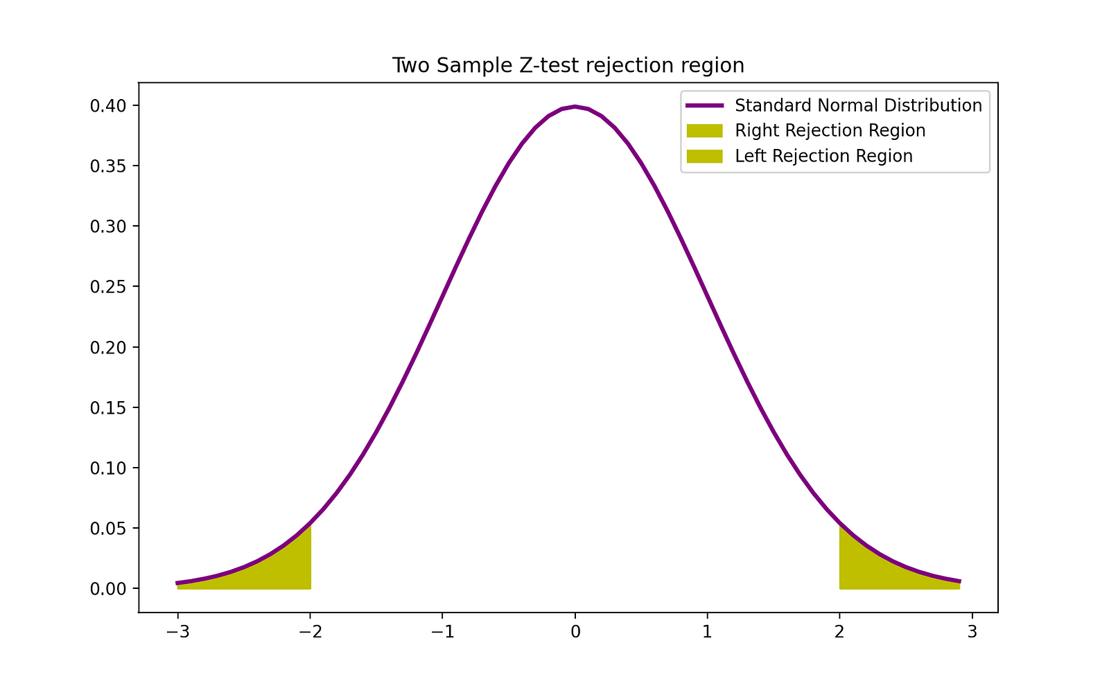
Image Source: The Author
The Python code snippet you’ve provided performs a two-sample Z-test for proportions. This type of test is used to determine whether there is a significant difference between the proportions of two groups. Here’s a brief explanation of the steps the code performs:
Calculates the sample proportions for both the control and experimental groups.
Computes the pooled sample proportion, which is an estimate of the proportion assuming the null hypothesis (that there is no difference between the group proportions) is true.
Calculates the pooled sample variance based on the pooled proportion and the sizes of the two samples.
Derives the standard error of the difference in sample proportions.
Calculates the Z-test statistic, which measures the number of standard errors between the sample proportion difference and the null hypothesis.
Finds the critical Z-value from the standard normal distribution for the given significance level.
Computes the p-value to assess the evidence against the null hypothesis.
Calculates the margin of error and the confidence interval for the difference in proportions.
Outputs the test statistic, critical value, p-value, and confidence interval, and based on the test statistic and critical value, it may print a statement to either reject or not reject the null hypothesis.
The latter part of the code uses Matplotlib to create a visualization of the standard normal distribution and the rejection regions for the two-sided Z-test. This visual aid helps to understand where the test statistic falls in relation to the distribution and the critical values.
import numpy as np
from scipy.stats import norm

X_con = 1242 #clicks control
N_con = 9886 #impressions control
X_exp = 974 #clicks experimental
N_exp = 10072 #impressions experimetal

# Significance Level
alpha = 0.05

p_con_hat = X_con / N_con
p_exp_hat = X_exp / N_exp

p_pooled_hat = (X_con + X_exp)/(N_con + N_exp)
pooled_variance = p_pooled_hat*(1-p_pooled_hat) * (1/N_con + 1/N_exp)

# Standard Error
SE = np.sqrt(pooled_variance)

# test statsitics
Test_stat = (p_con_hat - p_exp_hat)/SE
# critical value usig the standard normal distribution
Z_crit = norm.ppf(1-alpha/2)

# Margin of error
m = SE * Z_crit
# two sided test and using symmetry property of Normal distibution so we multiple with 2
p_value = norm.sf(Test_stat)*2

# Confidence Interval
CI = [(p_con_hat-p_exp_hat) - SE * Z_crit, (p_con_hat-p_exp_hat) + SE * Z_crit]

if np.abs(Test_stat) >= Z_crit:
    print("reject the null")
    print(p_value)

print("Test Statistics stat: ", Test_stat)
print("Z-critical: ", Z_crit)
print("P_value: ", p_value)
print("Confidence Interval of 2 sample Z-test for proportions: ", np.round(CI,2))

import matplotlib.pyplot as plt
z = np.arange(-3,3,  0.1)
plt.plot(z, norm.pdf(z), label = 'Standard Normal Distribution',color = 'purple',linewidth = 2.5)
plt.fill_between(z[z>Z_crit], norm.pdf(z[z>Z_crit]), label = 'Right Rejection Region',color ='y' )
plt.fill_between(z[z<(-1)*Z_crit], norm.pdf(z[z<(-1)*Z_crit]), label = 'Left Rejection Region',color ='y' )
plt.title("Two Sample Z-test rejection region")
plt.legend()
plt.show()
Case 2: Z-test for Comparing Means (2-sided)
If you want to test whether there is a statistically significant difference between the Control and Experimental groups’ metrics that are in the form of averages (like average purchase amount) you can use a 2-sample Z-test to test the following hypothesis:
$$\begin{cases} H_0: {CR}{\text{con}} = {CR}{\text{exp}} \\ H_1:{CR}{\text{con}} \neq {CR}{\text{exp}} \end{cases}$$
$$\begin{cases} H_0: {CR}{\text{con}} - {CR}{\text{exp}} = 0 \\ H_1: {CR}{\text{con}} - {CR}{\text{exp}} \neq 0 \end{cases}$$
where the sampling distribution of means of the Control group follows Normal distribution with mean mu_con and σ²_con/N_con. Moreover, the sampling distribution of means of the Experimental group also follows the Normal distribution with mean mu_exp and σ²_exp/N_exp.
$$\hat{\mu}{\text{con}} \sim N(\mu{con}, \frac{\sigma^2_{con}}{N_{con}})$$
$$\hat{\mu}{\text{exp}} \sim N(\mu{exp}, \frac{\sigma^{exp}2}{N{exp}})$$
Then the difference in the means of the control and experimental groups also follows Normal distributions with mean mu_con-mu_exp and variance σ²_con/N_con + σ²_exp/N_exp.
$$\hat{\mu}{\text{con}}-\hat{\mu}{\text{exp}} \sim N(\mu_{con}-\mu_{exp}, \frac{\sigma^2_{con}}{N_{con}}+\frac{\sigma^2_{exp}}{N_{exp}})$$
Consequently, the test statistics of the 2-sample Z-test for the difference in means can be calculated as follows:
$$T = \frac{\hat{\mu}{\text{con}}-\hat{\mu}{\text{exp}}}{\sqrt{\frac{\sigma^2_{con}}{N_{con}} + \frac{\sigma^2_{exp}}{N_{exp}}}} \sim N(0,1)$$
The Standard Error is equal to the square root of the estimate of the pooled variance and can be defined as:
$$SE = \sqrt{\frac{\sigma^2_{con}}{N_{con}} + \frac{\sigma^2_{exp}}{N_{exp}}}}$$
Then the p-value of this test statistics can be calculated as follows:
$$p_{\text{value}} = \Pr[Z \leq -T \text{ or } Z \geq T]$$
$$= 2 * \Pr[Z \geq T]$$
Finally, you can compute the Confidence Interval of the test as follows:
$$CI = [(\mu_hat_{con} - \mu_hat_{exp}) - z_{1-\alpha/2}*SE,((\mu_hat_{con} - \mu_hat_{exp}) + z_{1-\alpha/2)*SE]$$
The Python code provided appears to be set up for conducting a two-sample Z-test, typically used to determine if there is a significant difference between the means of two independent groups. In this context, the code might be comparing two different processes or treatments.
It generates two arrays of random integers to represent data for a control group (
X_A) and an experimental group (X_B).It calculates the sample means (
mu_con,mu_exp) and variances (variance_con,variance_exp) for both groups.The pooled variance is computed, which is used in the denominator of the test statistic formula for the Z-test, providing a measure of the data's common variance.
The Z-test statistic (
T) is calculated by taking the difference between the two sample means and dividing it by the standard error of the difference.The p-value is calculated to test the hypothesis of whether the means of the two groups are statistically different from each other.
The critical Z-value (
Z_crit) is determined from the standard normal distribution, which defines the cutoff points for significance.A margin of error is computed, and a confidence interval for the difference in means is constructed.
The test statistic, critical value, p-value, and confidence interval are printed to the console.
Lastly, the code uses Matplotlib to plot the standard normal distribution and highlight the rejection regions for the Z-test. This visualization can help in understanding the result of the Z-test in terms of where the test statistic lies relative to the distribution and the critical values for a two-sided test.
import numpy as np
from scipy.stats import norm

N_con = 60
N_exp = 60

# Significance Level
alpha = 0.05

X_A = np.random.randint(100, size = N_con)
X_B = np.random.randint(100, size = N_exp)

# Calculating means of control and experimental groups
mu_con = np.mean(X_A)
mu_exp = np.mean(X_B)

variance_con = np.var(X_A)
variance_exp = np.var(X_B)

# Pooled Variance
pooled_variance = np.sqrt(variance_con/N_con + variance_exp/N_exp)

# Test statistics
T = (mu_con-mu_exp)/np.sqrt(variance_con/N_con + variance_exp/N_exp)

# two sided test and using symmetry property of Normal distibution so we multiple with 2
p_value = norm.sf(T)*2

# Z-critical value
Z_crit  = norm.ppf(1-alpha/2)

# Margin of error
m = Z_crit*pooled_variance

# Confidence Interval
CI = [(mu_con - mu_exp) - m, (mu_con - mu_exp) + m]


print("Test Statistics stat: ", T)
print("Z-critical: ", Z_crit)
print("P_value: ", p_value)
print("Confidence Interval of 2 sample Z-test for proportions: ", np.round(CI,2))

import matplotlib.pyplot as plt
z = np.arange(-3,3,  0.1)
plt.plot(z, norm.pdf(z), label = 'Standard Normal Distribution',color = 'purple',linewidth = 2.5)
plt.fill_between(z[z>Z_crit], norm.pdf(z[z>Z_crit]), label = 'Right Rejection Region',color ='y' )
plt.fill_between(z[z<(-1)*Z_crit], norm.pdf(z[z<(-1)*Z_crit]), label = 'Left Rejection Region',color ='y' )
plt.title("Two Sample Z-test rejection region")
plt.legend()
plt.show()
Chi-Squared test
If you want to test whether there is a statistically significant difference between the Control and Experimental groups’ performance metrics (for example their conversions) and you don’t really want to know the nature of this relationship (which one is better) you can use a Chi-Squared test to test the following hypothesis:
$$\begin{cases} H_0: \CR_{\text{con}} = \CR_{\text{exp}} \\ H_1: \CR_{\text{con}} \neq \CR_{\text{exp}} \end{cases}$$
$$\begin{cases} H_0: \CR_{\text{con}} - \CR_{\text{exp}} = 0 \\ H_1: \CR_{\text{con}} - \CR_{\text{exp}} \neq 0 \end{cases}$$
Note that the metric should be in the form of a binary variable (for example, conversion or no conversion/click or no click). The data can then be represented in the form of the following table, where O and T correspond to observed and theoretical values, respectively.
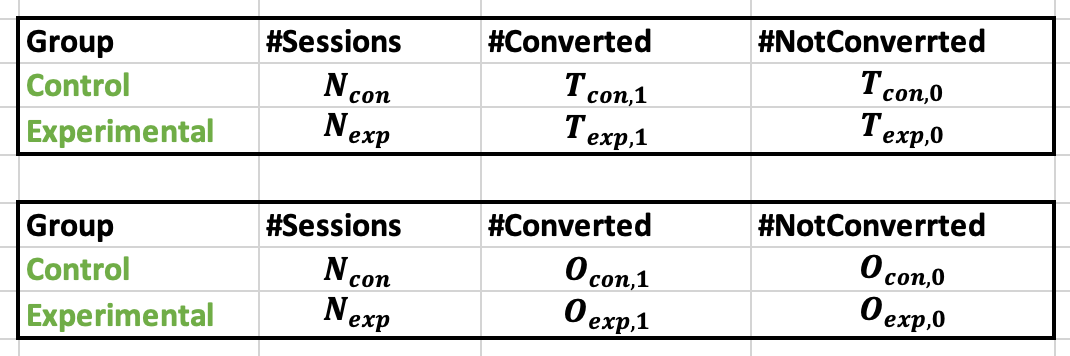
Table showing the data from Chi-Squared test
Then the test statistics of the Chi-2 test can be expressed as follows:
$$T = \sum_{i} \frac{(Observed_i - Expected_i)^2}{Expected_i}$$
where the Observed corresponds to the observed data and the Expected corresponds to the theoretical value, and i can take values 0 (no conversion) and 1(conversion). It’s important to see that each of these factors has a separate denominator. The formula for the test statistics when you have two groups only can be represented as follows:
$$T = \frac{(Observed_{con,1} - T_{con,1})^2}{T_{con,1}} + \frac{(Observed_{con,0} - T_{con,0})^2}{T_{con,0}} + \frac{(Observed_{exp,1} - T_{exp,1})^2}{T_{exp,1}} + \frac{(Observed_{exp,0} - T_{exp,0})^2}{T_{exp,0}}$$
The expected value is simply equal to the number of times each version of the product is viewed multiplied by the probability of it leading to conversion (or to a click in case of CTR).
Note that, since the Chi-2 test is not a parametric test, its Standard Error and Confidence Interval can’t be calculated in a standard way as we did in the parametric Z-test or T-test.
The rejection region of this two-sided 2-sample Z-test can be visualized by the following graph:
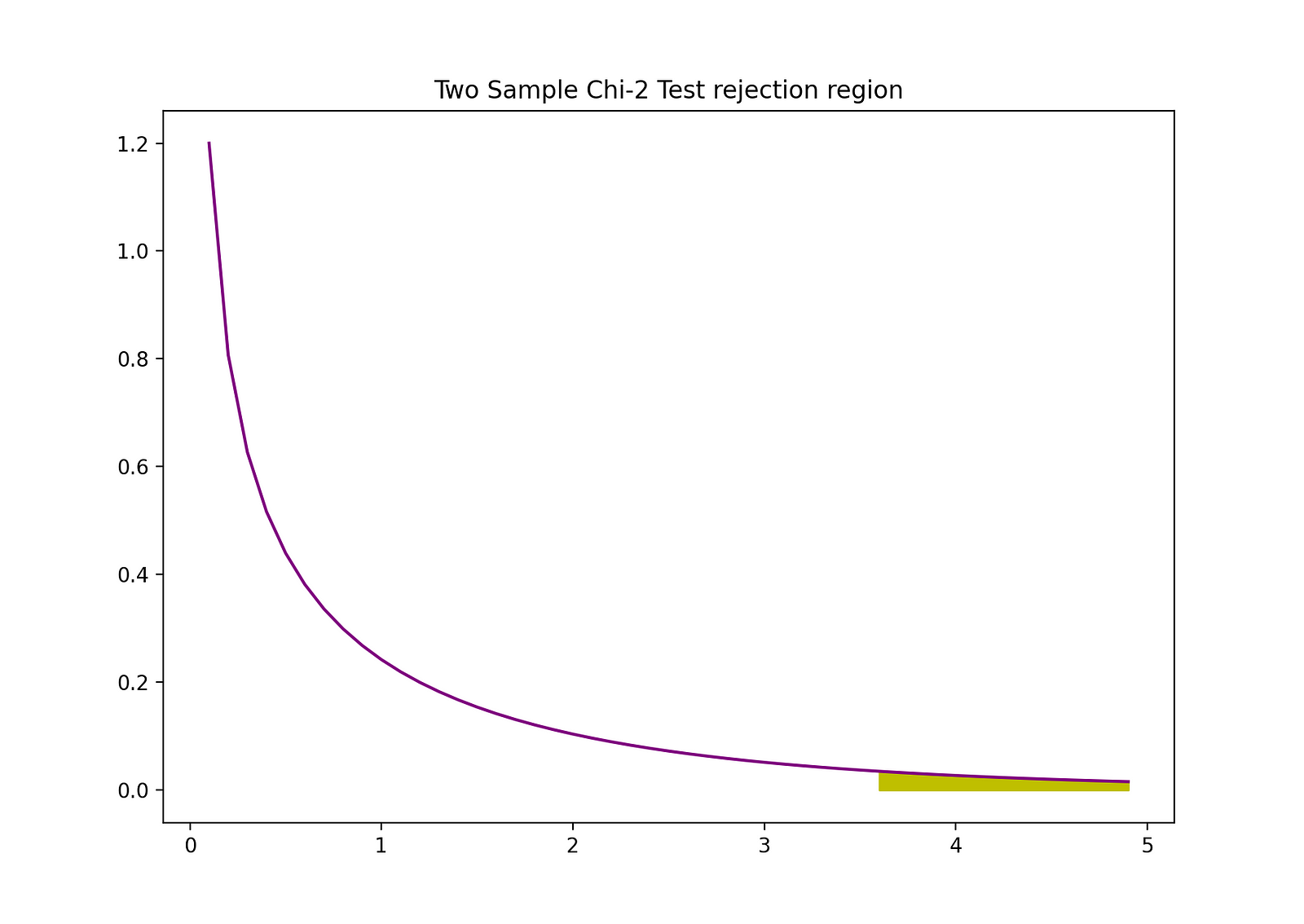
Image Source: The Author
The Python code you've shared is for conducting a Chi-squared test, a statistical hypothesis test that is used to determine whether there is a significant difference between the expected frequencies and the observed frequencies in one or more categories.
In the provided code snippet, it looks like the test is being used to compare two categorical datasets:
It calculates the Chi-squared test statistic by summing the squared difference between observed (
O) and expected (T) frequencies, divided by the expected frequencies for each category. This is known as the squared relative distance and is used as the test statistic for the Chi-squared test.It then calculates the p-value for this test statistic using the degrees of freedom, which in this case is assumed to be 1 (but this would typically depend on the number of categories minus one).
The Matplotlib library is used to plot the probability density function (pdf) of the Chi-squared distribution with one degree of freedom. It also highlights the rejection region for the test, which corresponds to the critical value of the Chi-squared distribution that the test statistic must exceed for the difference to be considered statistically significant.
The visualization helps to understand the Chi-squared test by showing where the test statistic lies in relation to the Chi-squared distribution and its critical value. If the test statistic is within the rejection region, the null hypothesis of no difference in frequencies can be rejected.
import numpy as np
from scipy.stats import chi2

O = np.array([86, 83, 5810,3920])
T = np.array([105,65,5781, 3841])

# Squared_relative_distance

def calculate_D(O,T):
    D_sum = 0
    for i in range(len(O)):
        D_sum += (O[i] - T[i])**2/T[i]
    return(D_sum)

D = calculate_D(O,T)
p_value = chi2.sf(D, df = 1)


import matplotlib.pyplot as plt
# Step 1: pick a x-axis range like in case of z-test (-3,3,0.1)
d = np.arange(0,5,0.1)
# Step 2: drawing the initial pdf of chi-2 with df = 1 and x-axis d range we just created
plt.plot(d, chi2.pdf(d, df = 1), color = "purple")
# Step 3: filling in the rejection region
plt.fill_between(d[d>D], chi2.pdf(d[d>D], df = 1), color = "y")
# Step 4: adding title
plt.title("Two Sample Chi-2 Test rejection region")
# Step 5: showing the plt graph
plt.show()
P-Values
Another quick way to determine whether to reject or to support the Null Hypothesis is by using p-values. The p-value is the probability of the condition under the Null occurring. Stated differently, the p-value is the probability, assuming the null hypothesis is true, of observing a result at least as extreme as the test statistic. The smaller the p-value, the stronger is the evidence against the Null Hypothesis, suggesting that it can be rejected.
The interpretation of a p-value is dependent on the chosen significance level. Most often, 1%, 5%, or 10% significance levels are used to interpret the p-value. So, instead of using the t-test and the F-test, p-values of these test statistics can be used to test the same hypotheses.
The following figure shows a sample output of an OLS regression with two independent variables. In this table, the p-value of the t-test, testing the statistical significance of class_size variable’s parameter estimate, and the p-value of the F-test, testing the joint statistical significance of the class_size, and el_pct variables parameter estimates, are underlined.
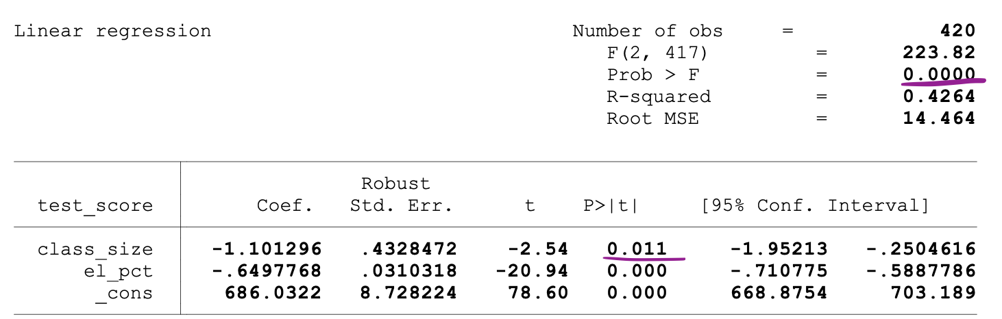
_Image Source:[ Stock and Whatson](https://www.uio.no/studier/emner/sv/oekonomi/ECON4150/v18/lecture7_ols_multiple_regressors_hypothesis_tests.pdf" data-href="https://www.uio.no/studier/emner/sv/oekonomi/ECON4150/v18/lecture7_ols_multiple_regressors_hypothesis_tests.pdf" class="markup--anchor markup--figure-anchor" rel="noopener" target="blank)
The p-value corresponding to the class_size variable is 0.011. When we compare this value to the significance levels 1% or 0.01 , 5% or 0.05, 10% or 0.1, then we can make the following conclusions:
0.011 > 0.01 → Null of the t-test can’t be rejected at 1% significance level
0.011 < 0.05 → Null of the t-test can be rejected at 5% significance level
0.011 < 0.10 → Null of the t-test can be rejected at 10% significance level
So, this p-value suggests that the coefficient of the class_size variable is statistically significant at 5% and 10% significance levels. The p-value corresponding to the F-test is 0.0000. And since 0 is smaller than all three cutoff values (0.01, 0.05, 0.10), we can conclude that the Null of the F-test can be rejected in all three cases.
This suggests that the coefficients of class_size and el_pct variables are jointly statistically significant at 1%, 5%, and 10% significance levels.
Limitation of p-values
Using p-values has many benefits, but it has also limitations. One of the main ones is that the p-value depends on both the magnitude of association and the sample size. If the magnitude of the effect is small and statistically insignificant, the p-value might still show a significant impact because the sample size is large. The opposite can occur as well – an effect can be large, but fail to meet the p<0.01, 0.05, or 0.10 criteria if the sample size is small.
Inferential Statistics
Inferential statistics uses sample data to make reasonable judgments about the population from which the sample data originated. We use it to investigate the relationships between variables within a sample and make predictions about how these variables will relate to a larger population.
Both the Law of Large Numbers (LLN) and the Central Limit Theorem (CLM) have a significant role in Inferential statistics because they show that the experimental results hold regardless of what shape the original population distribution was when the data is large enough.
The more data is gathered, the more accurate the statistical inferences become – hence, the more accurate parameter estimates are generated.
Law of Large Numbers (LLN)
Suppose X1, X2, . . . , Xn are all independent random variables with the same underlying distribution (also called independent identically-distributed or i.i.d), where all X’s have the same mean μ and standard deviation σ. As the sample size grows, the probability that the average of all X’s is equal to the mean μ is equal to 1.
The Law of Large Numbers can be summarized as follows:

Central Limit Theorem (CLM)
Suppose X1, X2, . . . , Xn are all independent random variables with the same underlying distribution (also called independent identically-distributed or i.i.d), where all X’s have the same mean μ and standard deviation σ. As the sample size grows, the probability distribution of X converges in the distribution in Normal distribution with mean μ and variance **σ-**squared.
The Central Limit Theorem can be summarized as follows:

Stated differently, when you have a population with mean μ and standard deviation σ and you take sufficiently large random samples from that population with replacement, then the distribution of the sample means will be approximately normally distributed.
Dimensionality Reduction Techniques
Dimensionality reduction is the transformation of data from a high-dimensional space into a low-dimensional space such that this low-dimensional representation of the data still contains the meaningful properties of the original data as much as possible.
With the increase in popularity in Big Data, the demand for these dimensionality reduction techniques, reducing the amount of unnecessary data and features, increased as well. Examples of popular dimensionality reduction techniques are Principle Component Analysis, Factor Analysis, Canonical Correlation, Random Forest.
Principle Component Analysis (PCA)
Principal Component Analysis (PCA) is a dimensionality reduction technique that is very often used to reduce the dimensionality of large data sets. It does this by transforming a large set of variables into a smaller set that still contains most of the information or the variation in the original large dataset.
Let’s assume we have a data X with p variables X1, X2, …., Xp with eigenvectors e1, …, ep, and eigenvalues λ1,…, λp. Eigenvalues show the variance explained by a particular data field out of the total variance.
The idea behind PCA is to create new (independent) variables, called Principal Components, that are a linear combination of the existing variable. The i_th_ principal component can be expressed as follows:
$$Y_i = e_{i1}X_1 + e_{i2}X_2 + e_{i3}X_3 + ... + e_{ip}X_p$$
Then using the Elbow Rule or Kaiser Rule, you can determine the number of principal components that optimally summarize the data without losing too much information.
It is also important to look at the proportion of total variation (PRTV) that is explained by each principal component to decide whether it is beneficial to include or to exclude it. PRTV for the i_th_ principal component can be calculated using eigenvalues as follows:
$$PRTV_i = \frac{{\lambda_i}}{{\sum_{k=1}^{p} \lambda_k}}$$
Elbow Rule
The elbow rule or the elbow method is a heuristic approach that we can use to determine the number of optimal principal components from the PCA results.
The idea behind this method is to plot the explained variation as a function of the number of components and pick the elbow of the curve as the number of optimal principal components.
Following is an example of such a scatter plot where the PRTV (Y-axis) is plotted on the number of principal components (X-axis). The elbow corresponds to the X-axis value 2, which suggests that the number of optimal principal components is 2.
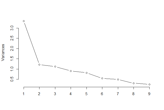
Image Source: [Multivariate Statistics Github](https://raw.githubusercontent.com/TatevKaren/Multivariate-Statistics/main/Elbow_rule%25varc_explained.png" data-href="https://raw.githubusercontent.com/TatevKaren/Multivariate-Statistics/main/Elbow_rule_%25varc_explained.png" class="markup--anchor markup--figure-anchor" rel="noopener" target="blank)
Factor Analysis (FA)
Factor analysis or FA is another statistical method for dimensionality reduction. It is one of the most commonly used inter-dependency techniques. We can use it when the relevant set of variables shows a systematic inter-dependence and our objective is to find out the latent factors that create a commonality.
Let’s assume we have a data X with p variables X1, X2, …., Xp. The FA model can be expressed as follows:
$$X-\mu = AF + u$$
where:
X is a [p x N] matrix of p variables and N observations
µ is [p x N] population mean matrix
A is [p x k] common factor loadings matrix
F [k x N] is the matrix of common factors
and u [pxN] is the matrix of specific factors.
So, to put it differently, a factor model is as a series of multiple regressions, predicting each of the variables Xi from the values of the unobservable common factors are:
$$X_1 = \mu_1 + a_{11}f_1 + a_{12}f_2 + ... + a_{1m}f_m + u1\\ X_2 = \mu_2 + a_{21}f_1 + a_{22}f_2 + ... + a_{2m}f_m + u2\\ .\\ .\\ .\\ X_p = \mu_p + a_{p1}f_1 + a_{p2}f_2 + ... + a_{pm}f_m + up$$
Each variable has k of its own common factors, and these are related to the observations via the factor loading matrix for a single observation as follows:
In factor analysis, the factors are calculated to maximize between-group variance while minimizing in-group variance. They are factors because they group the underlying variables. Unlike the PCA, in FA the data needs to be normalized, given that FA assumes that the dataset follows Normal Distribution.
Interview Prep – Top 7 Statistics Questions with Answers
Are you preparing for interviews in statistics, data analysis, or data science? It's crucial to know key statistical concepts and their applications.
Below I've included seven important statistics questions with answers, covering basic statistical tests, probability theory, and the use of statistics in decision-making, like A/B testing.
Question 1: What is the difference between a t-test and Z-test?
The question "What is the difference between a t-test and Z-test?" is a common question in data science interviews because it tests the candidate's understanding of basic statistical concepts used in comparing group means.
This knowledge is crucial because choosing the right test affects the validity of conclusions drawn from data, which is a daily task in a data scientist's role when it comes to interpreting experiments, analyzing survey results, or evaluating models.
Answer:
Both t-tests and Z-tests are statistical methods used to determine if there are significant differences between the means of two groups. But they have key differences:
Assumptions: You can use a t-test when the sample sizes are small and the population standard deviation is unknown. It doesn't require the sample mean to be normally distributed if the sample size is sufficiently large due to the Central Limit Theorem. The Z-test assumes that both the sample and the population distributions are normally distributed.
Sample Size: T-tests are typically used for sample sizes smaller than 30, whereas Z-tests are used for larger sample sizes (greater than or equal to 30) when the population standard deviation is known.
Test Statistic: The t-test uses the t-distribution to calculate the test statistic, taking into account the sample standard deviation. The Z-test uses the standard normal distribution, utilizing the known population standard deviation.
P-Value: The p-value in a t-test is determined based on the t-distribution, which accounts for the variability in smaller samples. The Z-test uses the standard normal distribution to calculate the p-value, suitable for larger samples or known population parameters.
Question 2: What is a p-value?
The question "What is a p-value?" requires the understanding of a fundamental concept in hypothesis testing that we descussed in this blog in detail with examples. It's not just a number – it's a bridge between the data you collect and the conclusions you draw for data driven decision making.
P-values quantify the evidence against a null hypothesis—how likely it is to observe the collected data if the null hypothesis were true.
For data scientists, p-values are part of everyday language in statistical analysis, model validation, and experimental design. They have to interpret p-values correctly to make informed decisions and often need to explain their implications to stakeholders who might not have deep statistical knowledge.
Thus, understanding p-values helps data scientists to convey the level of certainty or doubt in their findings and to justify subsequent actions or recommendations.
So here you need to show your understanding of what p-value measures and connect it to statistical significance and hypothesis testing.
Answer:
The p-value measures the probability of observing a test statistic at least as extreme as the one observed, under the assumption that the null hypothesis is true. It helps in deciding whether the observed data significantly deviate from what would be expected under the null hypothesis.
If the p-value is lower than a predetermined threshold (alpha level, usually set at 0.05), the null hypothesis is rejected, indicating that the observed result is statistically significant.
Question 3: What are limitations of p-values?
P-values are a staple of inferential statistics, providing a metric for evaluating evidence against a null hypothesis. In these question you need to name couple of them.
Answer
Dependence on Sample Size: The p-value is sensitive to the sample size. Large samples might yield significant p-values even for trivial effects, while small samples may not detect significant effects even if they exist.
Not a Measure of Effect Size or Importance: A small p-value does not necessarily mean the effect is practically significant – it simply indicates it's unlikely to have occurred by chance.
Misinterpretation: P-values can be misinterpreted as the probability that the null hypothesis is true, which is incorrect. They only measure the evidence against the null hypothesis.
Question 4: What is a Confidence Level?
A confidence level represents the frequency with which an estimated confidence interval would contain the true population parameter if the same process were repeated multiple times.
For example, a 95% confidence level means that if the study were repeated 100 times, approximately 95 of the confidence intervals calculated from those studies would be expected to contain the true population parameter.
Question 5: What is the Probability of Picking 5 Red and 5 Blue Balls Without Replacement?
What is the probability of picking exactly 5 red balls and 5 blue balls in 10 picks without replacement from a set of 100 balls, where there are 70 red balls and 30 blue balls? The text describes how to calculate this probability using combinatorial mathematics and the hypergeometric distribution.
In this question, you're dealing with a classic probability problem that involves combinatorial principles and the concept of probability without replacement. The context is a finite set of balls, each draw affecting the subsequent ones because the composition of the set changes with each draw.
To approach this problem, you need to consider:
The total number of balls: If the question doesn't specify this, you need to ask or make a reasonable assumption based on the context.
Initial proportion of balls: Know the initial count of red and blue balls in the set.
Sequential probability: Remember that each time you draw a ball, you don't put it back, so the probability of drawing a ball of a certain color changes with each draw.
Combinations: Calculate the number of ways to choose 5 red balls from the total red balls and 5 blue balls from the total blue balls, then divide by the number of ways to choose any 10 balls from the total.
Thinking through these points will guide you in formulating the solution based on the hypergeometric distribution, which describes the probability of a given number of successes in draws without replacement from a finite population.
This question tests your ability to apply probability theory to a dynamic scenario, a skill that's invaluable in data-driven decision-making and statistical modeling.
Answer:
To find the probability of picking exactly 5 red balls and 5 blue balls in 10 picks without replacement, we calculate the probability of picking 5 red balls out of 70 and 5 blue balls out of 30, and then divide by the total ways to pick 10 balls out of 100:

Let's calculate this probability:

Question 6: Explain Bayes' Theorem and its importance in calculating posterior probabilities.
Provide an example of how it might be used in genetic testing to determine the likelihood of an individual carrying a certain gene.
Bayes' Theorem is a cornerstone of probability theory that enables the updating of initial beliefs (prior probabilities) with new evidence to obtain updated beliefs (posterior probabilities). This question wants to test candidates ability to explain the concept, mathematical framework for incorporating new evidence into existing predictions or models.
Answer:
Bayes' Theorem is a fundamental theorem in probability theory and statistics that describes the probability of an event, based on prior knowledge of conditions that might be related to the event. It's crucial for calculating posterior probabilities, which are the probabilities of hypotheses given observed evidence.

P(A_∣_B) is the posterior probability: the probability of hypothesis A given the evidence B.
P(B∣A) is the likelihood: the probability of observing evidence B given that hypothesis A is true.
P(A) is the prior probability: the initial probability of hypothesis A, before observing evidence B.
P(B) is the marginal probability: the total probability of observing evidence B_B_ under all possible hypotheses.
Question 7: Describe how you would statistically determine if the results of an A/B test are significant - walk me through AB Testing process.
In this question, the interviewer is assessing your comprehensive knowledge of the A/B testing framework. They are looking for evidence that you can navigate the full spectrum of A/B testing procedures, which is essential for data scientists and AI professionals tasked with optimizing features, making data-informed decisions, and testing software products.
The interviewer wants to confirm that you understand each step in the process, beginning with formulating statistical hypotheses derived from business objectives. They are interested in your ability to conduct a power analysis and discuss its components, including determining effect size, significance level, and power, all critical in calculating the minimum sample size needed to detect a true effect and prevent p-hacking.
The discussion on randomization, data collection, and monitoring checks whether you grasp how to maintain the integrity of the test conditions. You should also be prepared to explain the selection of appropriate statistical tests, calculation of test statistics, p-values, and interpretation of results for both statistical and practical significance.
Ultimately, the interviewer is testing whether you can act as a data advocate: someone who can meticulously run A/B tests, interpret the results, and communicate findings and recommendations effectively to stakeholders, thereby driving data-driven decision-making within the organization.
To Learn AB Testing check my AB Testing Crash Course on YouTube.
Answer:
In an A/B test, my first step is to establish clear business and statistical hypotheses. For example, if we’re testing a new webpage layout, the business hypothesis might be that the new layout increases user engagement. Statistically, this translates to expecting a higher mean engagement score for the new layout compared to the old.
Next, I’d conduct a power analysis. This involves deciding on an effect size that's practically significant for our business context—say, a 10% increase in engagement. I'd choose a significance level, commonly 0.05, and aim for a power of 80%, reducing the likelihood of Type II errors.
The power analysis, which takes into account the effect size, significance level, and power, helps determine the minimum sample size needed. This is crucial for ensuring that our test is adequately powered to detect the effect we care about and for avoiding p-hacking by committing to a sample size upfront.
With our sample size determined, I’d ensure proper randomization in assigning users to the control and test groups, to eliminate selection bias. During the test, I’d closely monitor data collection for any anomalies or necessary adjustments.
Upon completion of the data collection, I’d choose an appropriate statistical test based on the data distribution and variance homogeneity—typically a t-test if the sample size is small or a normal distribution can’t be assumed, or a Z-test for larger samples with a known variance.
Calculating the test statistic and the corresponding p-value allows us to test the null hypothesis. If the p-value is less than our chosen alpha level, we reject the null hypothesis, suggesting that the new layout has a statistically significant impact on engagement.
In addition to statistical significance, I’d evaluate the practical significance by looking at the confidence interval for the effect size and considering the business impact.
Finally, I’d document the entire process and results, then communicate them to stakeholders in a clear, non-technical language. This includes not just the statistical significance, but also how the results translate to business outcomes. As a data advocate, my goal is to support data-driven decisions that align with our business objectives and user experience strategy
For getting more interview questions from Stats to Deep Learning - with over 400 Q&A as well as personalized interview preparation check out our Free Resource Hub and our Data Science Bootcamp with Free Trial.
Thank you for choosing this guide as your learning companion. As you continue to explore the vast field of machine learning, I hope you do so with confidence, precision, and an innovative spirit. Best wishes in all your future endeavors!
About the Author
I am Tatev Aslanyan, Senior Machine Learning and AI Researcher, and Co-Founder of LunarTech where we are making Data Science and AI accessible to everyone. I have had the privilege of working in Data Science across numerous countries, including the US, UK, Canada, and the Netherlands.
With an MSc and BSc in Econometrics under my belt, my journey in Machine and AI has been nothing short of incredible. Drawing from my technical studies during my Bachelors & Masters, along with over 5 years of hands-on experience in the Data Science Industry, in Machine Learning and AI, I've gathered this high-level summary of ML topics to share with you.
How Can You Dive Deeper?
After studying this guide, if you're keen to dive even deeper and structured learning is your style, consider joining us at LunarTech, we offer individual courses and Bootcamp in Data Science, Machine Learning and AI.
We provide a comprehensive program that offers an in-depth understanding of the theory, hands-on practical implementation, extensive practice material, and tailored interview preparation to set you up for success at your own phase.
You can check out our Ultimate Data Science Bootcamp and join a free trial to try the content first hand. This has earned the recognition of being one of the Best Data Science Bootcamps of 2023, and has been featured in esteemed publications like Forbes, Yahoo, Entrepreneur and more. This is your chance to be a part of a community that thrives on innovation and knowledge. Here is the Welcome message!
Connect with Me

LunarTech Newsletter
Follow me on LinkedIn and on YouTube
Subscribe to my The Data Science and AI Newsletter
If you want to learn more about a career in Data Science, Machine Learning and AI, and learn how to secure a Data Science job, you can download this free Data Science and AI Career Handbook.