
By Joel Hereth
In the vast and ever-growing realm of data analytics, Structured Query Language (SQL) serves as a fundamental building block.
While SQL's roots lie in database management, it has expanded its reach, becoming the go-to tool for data extraction, manipulation, and analysis.
Whether you're just starting your journey as a data analyst or looking to bolster your proficiency in its tools, understanding essential SQL concepts is non-negotiable.
This guide will take you through the critical aspects of SQL that are important for your success in the data analytics field.
Table of Contents:
- The Role of SQL in Data Analytics
- Key SQL Concepts to Learn
– Basic Commands
– TheCASEStatement
– Subqueries and Common Table Expressions (CTEs)
– Joins and Unions
– String and Date Formatting
– Window Functions - Conclusion
The Role of SQL in Data Analytics
Before getting into the nitty-gritty, it's important to understand the pivotal role of SQL in data analytics.
SQL is the lingua franca of the database world, serving as a translator between human and machine. This makes it a must-learn for anyone diving into the data domain.
To appreciate SQL's significance, you need only to look at the tasks it allows you to perform. From transforming raw data into insightful reports to creating data-driven applications and executing complex data operations, SQL is the powerhouse that enables analysts and professionals to extract hidden gems from the vast seas of databases.
Key SQL Concepts to Learn
Basic Commands
SQL commands can be categorized into entities that manage the structure of the database schema (DDL - Data Definition Language), control the content of the database tables (DML - Data Manipulation Language), and access and work on the data within the database (DQL - Data Query Language). You'll want to start here to lay a solid foundation.
DML Commands:
SELECT: retrieves data from one or more tables.
SELECT product_name, price
FROM products
WHERE category = 'Electronics';
INSERT: inserts new rows into a table.
INSERT INTO customers (name, email)
VALUES ('John Doe', 'john@example.com');
UPDATE: modifies existing data within a table.
UPDATE inventory
SET quantity = 50
WHERE product_id = 101;
DELETE: removes existing rows from a table.
DELETE FROM orders
WHERE order_id = 12345;
DDL Commands:
CREATE TABLE: creates a new table within the database.
CREATE TABLE employees (
    employee_id INT PRIMARY KEY,
    name VARCHAR(50),
    department VARCHAR(50),
    salary DECIMAL(10, 2)
);
ALTER TABLE: modifies an existing table within the database.
ALTER TABLE employees
ADD hire_date DATE;
DROP TABLE: removes an entire table from the database.
DROP TABLE customers;
DQL Commands:
SELECT: also part of DML but often associated with DQL as it is used to query data only.
The CASE Statement
The CASE statement takes scalars, predicates, function calls, and even SQL queries as input and returns an expression value. It’s an extremely versatile tool that can be used to transform data, perform if-then-else logic, categorize information, and more.
Basic Syntax of CASE:
SELECT column_name,
  CASE
    WHEN condition1 THEN result1
    WHEN condition2 THEN result2
    ELSE result3
  END
FROM table_name;
Understanding how and when to use CASE statements is a critical SQL skill to master as a data analyst dealing with complex datasets. To showcase the different CASE statements, we have the actions table with the user_id, action, and date fields.
CREATE TABLE actions (
  "user_id" INTEGER,
  "action" VARCHAR(50),
  "date" DATE
);

INSERT INTO actions (
     "user_id",
      "action",
      "date"
)
VALUES
    (1, 'post', current_timestamp::DATE-3),
    (2, 'edit', current_timestamp::DATE-2),
    (3, 'post', current_timestamp::DATE-1),
    (4, 'post', current_timestamp::DATE-1),
    (5, 'edit', current_timestamp::DATE-5),
    (6, 'cancel', current_timestamp::DATE-2),
    (7, 'post', current_timestamp::DATE-2),
    (8, 'post', current_timestamp::DATE-1),
    (9, 'post', current_timestamp::DATE-1),
    (10, 'cancel', current_timestamp::DATE-3),
    (11, 'post', current_timestamp::DATE-2),
    (12, 'post', current_timestamp::DATE-2);
Your manager is about to go into a meeting with the event director and asks you to write a query to showcase the current post rate for all time rounded two decimals. In this case based on the actions table structure, we'll need to utilize a CASE statement.
select round(1.0*
sum(case when action='post' then 1 else 0 end)
/
count(1)
,2) post_rate
from actions;
Initially, we employ a CASE statement to assign a value of 1 to posts, and 0 otherwise. Afterward, we aggregate these results using SUM(). Then, we divide this sum by the total count of records, represented by COUNT(1), which includes all records, not exclusively posts.
This computation yields our post rate. To ensure decimal precision, we multiply the numerator by 1.0. Finally, we round the entire result to two decimal points as needed.
Subqueries and Common Table Expressions (CTEs)
Subqueries, or inner queries, allow you to use queries within another SQL statement. Common Table Expressions (CTEs) are named temporary result sets that you can reference within a SELECT, INSERT, UPDATE, or DELETE statement.
Subqueries:
- Scalar Subquery: a subquery that returns a single value.
- Column Subquery: a subquery that returns one or more columns.
- Table Subquery: a subquery that looks like a table (used with any operator expecting a table).
CTEs:
- Provide a more readable and maintainable alternative to a derived table or subquery.
- Can reference themselves, which is useful for recursive queries.
To demonstrate the use cases, we're going to practice with both the traditional subquery and CTE using the following SQL schema:
CREATE TABLE all_numbers (
  "phone_number" VARCHAR(25)
  );


CREATE TABLE confirmed_numbers (
  "phone_number" VARCHAR(25)
  );


INSERT INTO all_numbers
("phone_number")
VALUES
('706-766-8523'),
('555-239-6874'),
('407-234-5041'),
('(123)351-6123'),
('251-874-3478');

INSERT INTO confirmed_numbers
 ("phone_number")
 VALUES
('555-239-6874'),
('407-234-5041'),
('(123)351-6123');
For example, let's say you're a data analyst at DoorDash and you've been asked to retrieve all the phone numbers that are in the all_numbers table but are not present in the confirmed_numbers table. You can solve this by using a traditional subquery:
SELECT phone_number
FROM all_numbers
WHERE phone_number NOT IN (
  SELECT phone_number
  FROM confirmed_numbers
);
Alternatively, if the database is very large, you might want to think about using a CTE since they're more efficient for larger databases.
WITH excluded_numbers AS (
  SELECT phone_number
  FROM confirmed_numbers
)

SELECT phone_number
FROM all_numbers
WHERE phone_number NOT IN (
  SELECT phone_number
  FROM excluded_numbers
);
Joins and Unions
Joins help you combine data from multiple tables based on a related column between them, while unions allow you to combine the result sets of two or more SELECT statements. Both are critical for harnessing the full power of your SQL queries.
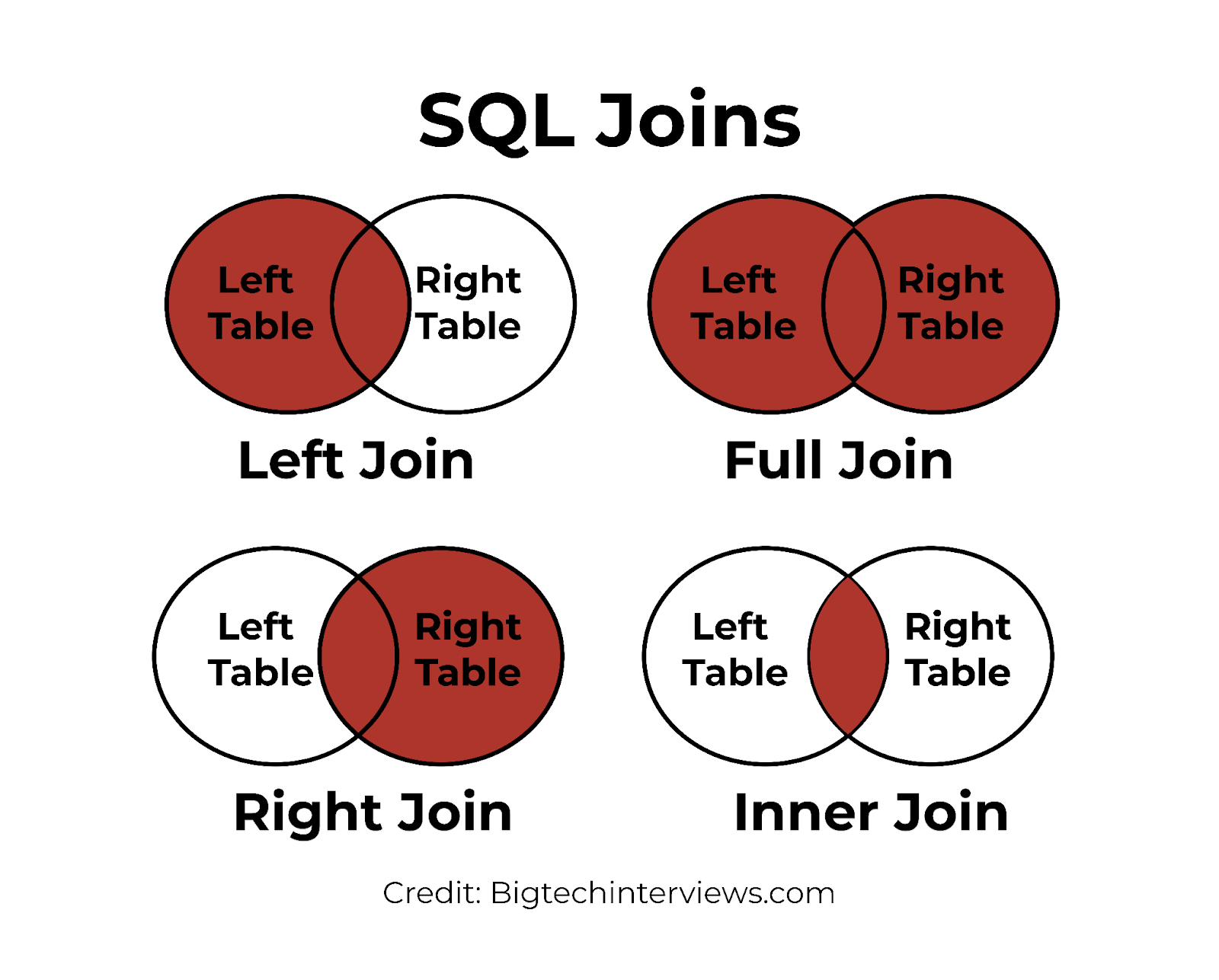
Types of Joins:
INNER JOIN: returns rows when there is a match in both tables.LEFT JOIN: returns all rows from the left table and the matched rows from the right table.RIGHT JOIN: returns all rows from the right table and the matched rows from the left table.FULL JOIN: returns all rows when there is a match in one of the tables.
To illustrate the various JOIN types in SQL, consider a scenario where we want to compile the relationship between sales figures and their corresponding sales representatives across different regions.
For this purpose, we have two tables: sales_data and representatives. They are linked by the rep_id field, which serves as a foreign key in the sales_data table and a primary key in the representatives table. Here's what that looks like:
CREATE TABLE sales_data (
    sale_id INT PRIMARY KEY,
    rep_id INT,
    region VARCHAR(50),
    sales DECIMAL(10, 2)
);

INSERT INTO sales_data (sale_id, rep_id, region, sales) VALUES
(1, 101, 'East', 1000.00),
(2, 102, 'East', 1500.50),
(3, 103, 'West', 2000.00),
(4, 104, 'West', 2500.75),
(5, NULL, 'West', 3000.00);

CREATE TABLE representatives (
    rep_id INT PRIMARY KEY,
    sales_rep VARCHAR(100),
    region VARCHAR(50)
);
INSERT INTO representatives (rep_id, sales_rep, region) VALUES
(101, 'John Doe', 'East'),
(102, 'Jane Smith', 'East'),
(105, 'Jim Beam', 'North'),
(106, 'Jill Jackson', 'North'),
(107, 'Jack Johnson', 'South');
For our example, suppose we want to match sales to representatives in the East region. We would use an INNER JOIN to fetch only the rows with matching rep_id in both tables:
SELECT s.sales, r.sales_rep
FROM sales_data s
INNER JOIN representatives r
ON s.rep_id = r.rep_id
WHERE s.region = 'East';
In the case of wanting to see all sales data in the West region, including those without a corresponding sales representative, a LEFT JOIN comes in handy:
SELECT s.sales, r.sales_rep
FROM sales_data s
LEFT JOIN representatives r
ON s.rep_id = r.rep_id
WHERE s.region = 'West';
If our interest instead is in all representatives in the North region, even those without associated sales data, we would use a RIGHT JOIN:
SELECT s.sales, r.sales_rep
FROM sales_data s
RIGHT JOIN representatives r
ON s.rep_id = r.rep_id
WHERE r.region = 'North';
Lastly, to see all possible combinations of sales and representatives across all regions, regardless of matching rep_id, we use a FULL JOIN:
SELECT s.sales, r.sales_rep
FROM sales_data s
FULL JOIN representatives r
ON s.rep_id = r.rep_id;
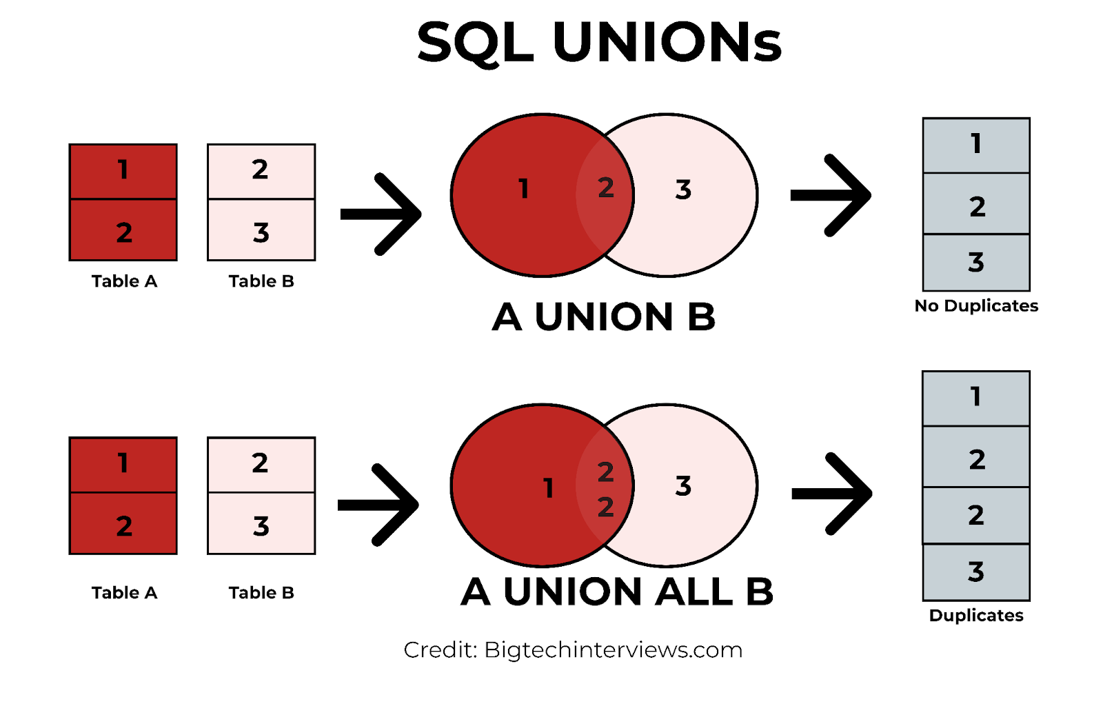
Union and Union All:
UNION: returns the distinct rows that appear in either of the two result sets.UNION ALL: returns all the rows including duplicates.
Continuing with the same SQL schema above containing the sales_data table and representatives table, let's review scenarios where we'd want use a UNION and UNION ALL.
Using a UNION, let's construct a SQL query to efficiently retrieve the names of all sales representatives from both the sales_data and representatives tables.
SELECT sales_rep AS representative_name FROM representatives
UNION
SELECT DISTINCT rep_id AS representative_name FROM sales_data;
Now, let's explore how to utilize a UNION ALL operation to retrieve the names of all sales representatives from both the sales_data and representatives tables, including duplicates.
SELECT sales_rep AS representative_name FROM representatives
UNION ALL
SELECT DISTINCT rep_id AS representative_name FROM sales_data;
String and Date Formatting
The manipulation of string and date values is common in data analysis. Understanding how to format these types properly is crucial for meaningful analysis.
String Functions:
CONCAT: merges two or more strings into one.SUBSTRING: returns a part of a string.LENGTHorLEN: returns the length of a string.
Date Functions:
DATEADD: adds an interval to a date.DATEDIFF: returns the time between two dates.DATENAMEorTO_CHAR: Returns part of a date like day, month, or year.
To demonstrate the usage of string and date functions in SQL, let's delve into a scenario involving orders and deliveries.
We have two tables: orders and deliveries. Here's a breakdown of each table and its columns:
CREATE TABLE orders (
    order_id INT PRIMARY KEY,
    customer_id INT,
    order_date DATE,
    total_amount DECIMAL(10, 2)
);

INSERT INTO orders (order_id, customer_id, order_date, total_amount) VALUES
(1, 201, '2024-02-20', 500.00),
(2, 202, '2024-02-21', 750.25),
(3, 203, '2024-02-21', 1000.00),
(4, 204, '2024-02-22', 1200.75),
(5, 205, '2024-02-22', 1500.00);

CREATE TABLE deliveries (
    delivery_id INT PRIMARY KEY,
    order_id INT,
    delivery_date DATE,
    delivery_status VARCHAR(50)
);

INSERT INTO deliveries (delivery_id, order_id, delivery_date, delivery_status) VALUES
(1, 1, '2024-02-21', 'Delivered'),
(2, 2, '2024-02-22', 'In transit'),
(3, 3, '2024-02-22', 'Delivered'),
(4, 4, NULL, 'Pending'),
(5, 5, NULL, 'Pending');
Say you've been tasked with optimizing order tracking systems. To streamline this process, you need to create unique order identifiers by merging customer IDs and order IDs. Leveraging the CONCAT function in SQL, you merge these identifiers, ensuring efficient order management and analysis.
SELECT CONCAT(customer_id, '-', order_id) AS order_identifier
FROM orders;
Your next task is to categorize delivery statuses accurately, which is essential for operational efficiency. But delivery status messages often contain irrelevant details.
To simplify this process, you use the SUBSTRING function in SQL to extract the initial characters of the delivery status. This enables swift categorization and analysis of delivery progress.
SELECT SUBSTRING(delivery_status, 1, 3) AS status_summary
FROM deliveries;
Now imagine you need to ensure the consistency of delivery status messages. It's crucial to validate that delivery status updates adhere to defined length constraints.
By employing the LENGTH/LEN function in SQL, you calculate the length of each delivery status message. This facilitates robust validation mechanisms, ensuring uniformity and integrity in your data.
SELECT delivery_id, LENGTH(delivery_status) AS status_length
FROM deliveries;
Date Functions
When querying the orders and deliveries tables in the SQL schema provided, the DATEADD function is particularly useful in scenarios where you need to calculate future dates or deadlines based on existing ones.
For example, you might use DATEADD to find the expected delivery date by adding a certain number of days to order_date to ensure delivery within a predefined time frame.
SELECT order_id, customer_id, DATEADD(day, 3, order_date) AS expected_delivery_date
FROM orders;
The DATEDIFF function can also be useful in calculating differences between dates. For instance, if you need to find the average time it takes for an order to be delivered, you could subtract the order_date from the delivery_date and then calculate the average using AVG.
SELECT AVG(DATEDIFF(day,order_date,delivery_date)) AS average_delivery_time
FROM orders o INNER JOIN deliveries d ON o.order_id = d.order_id
WHERE delivery_status = 'Delivered';
TO_CHAR function can be useful in converting dates to a specific format. For instance, if you need to display the delivery date as Month DD, YYYY instead of the default format, you could use TO_CHAR in your query.
SELECT order_id, customer_id, TO_CHAR(delivery_date,'Month DD, YYYY') AS formatted_delivery_date
FROM orders o INNER JOIN deliveries d ON o.order_id = d.order_id;
Window Functions
Window functions are a powerful feature that allow you to perform calculations across a set of table rows related to the current row, known as the window, without the need for a self-join. This includes the capability to perform running totals, moving averages, and more.
Common Window Functions:
ROW_NUMBER(): assigns a unique number to each row to which a window function is applied.RANK(): provides a rank to each row within a result set with the same rank given to the rows that have the same ranking.DENSE_RANK(): similar toRANK(), but the ranks are consecutive.
CREATE TABLE product_data (
    product_id INT PRIMARY KEY,
    total_inventory INT NOT NULL,
    total_sales INT NOT NULL,
    region VARCHAR(50) NOT NULL
);
INSERT INTO product_data (product_id, total_inventory, total_sales, region) VALUES
(1, 100, 500, 'North America'),
(2, 150, 750, 'Europe'),
(3, 200, 1000, 'Asia'),
(4, 120, 1200, 'North America'),
(5, 180, 1500, 'Europe');
For example, your sales director Slacks you and asks you to calculate a running total of sales over product inventory. You can do this using a basic SUM Window Function ()
SELECT
    product_id,
    total_inventory,
    SUM(total_sales) OVER(ORDER BY product_id) AS running_total_sales
FROM product_data;
Now, diving deeper into the problem. Say it's a large dataset and Excel won't cut it for this task and you want to partition it out by region. You can do this by applying ROW_NUMBER().
SELECT
    region,
    product_id,
    ROW_NUMBER() OVER(PARTITION BY region ORDER BY product_id) AS region_product_rank
FROM product_data;
Alternatively, you could swap the ROW_NUMBER() for DENSE_RANK() or RANK() depending on the the use case.
Conclusion
As a data analyst, your proficiency in SQL will evolve as you handle more complex data scenarios and questions.
These essential SQL concepts serve as a good starting point – but continuous learning and applying these concepts in practical scenarios are what will truly solidify your understanding and expertise.
Keep exploring new features, tools, and resources such freeCodeCamp or Big Tech Interviews, and you'll find SQL to be an ever-rewarding, ever-deepening skill to have in your data toolkit.